blog - Page 11 of 13 - yoursumbuddy

Conditional Formatting Digital Clock

Posted on May 23, 2012 by Doug Glancy

I was staring at a video player the other day and thinking about digital clocks, specifically, of course, digital clocks created in Excel. As I imagined, there are quite a few out there: Juan Pablo Gonzalez already had one on DDOE back in 2004, Andy Pope’s is indistinguishable from the real thing, and Tushar Mehta’s is accurate to within one nanosecond every three years. But as far as I can tell there aren’t any created using conditional formatting. Let me know if I’m wrong, but meanwhile here’s a conditional formatting digital clock in a live workbook.

As the notes in the worksheet above say, you can update this clock by clicking in a cell and hitting F9. Not very convenient, but the best I can do without macros. (See the download at the end for full automation). You can adjust the time to your location, instead of that of your server, with the “Hour Offset” setting. To see the full works click on the second worksheet tab.

My basic idea was to use conditional formatting cell borders to form the digits. Each digit would consist of two cells on top of each other.

The first issue was how to have doubled lines for cell borders. Conditional formatting doesn’t have this option. Regular cell borders do though, so the answer was to put double line borders around all the digit cells and then have the conditional formatting “erase” the unneeded ones.

The formatting feeds from this grid, which you can see on the second worksheet. Each clock digit is formed from two cells, the “top” and “bottom.” Each of the four borders for each cell has a 0 or 1 setting.

I originally had the table rows filled with 1, 2, 4 and 8 for each cell, thinking to roll the four numbers up into something like a composite enumerated value. Then I tried to use Mod to parse the rolled-up result for each half-digit. If that sounds confusing, it should! I eventually realized that since I essentially needed to determine if each border’s “bit” was on or off, I should just use a table with zeros and ones.

The conditional formatting formula, listed below, finds the relevant digit and it’s top or bottom position and checks whether it’s set to 0. If so, the conditional formatting “erases” the existing border. Otherwise the original double border is left in place.

There are actually four very similar formulas. The only thing that changes is the …”,1)=0″ part at the end. That’s checking the first column, i.e., the left border. The other formulas check, the 2nd, 3rd and 4th columns (the top, bottom and right borders).

=INDEX($R$6:$U$25,
SUMPRODUCT(
($P$6:$P$25=$S1)*
($Q$6:$Q$25=(MID($T$1,((COLUMNS($A:A)+1)/2),1)))*
(ROW($P$6:$P$25)-ROW($P$5)))
,1)
=0

It’s a two-dimensional Index formula. The most interesting thing is that the row dimension is determined by a Sumproduct formula, which finds the row that has the correct digit and top or bottom position. I’ll try to do a short post on this sometime, or if anybody has a good link, let me know.

This digital clock requires Excel 2007 or 2010 because there are four conditions per cell, and Excel 2003 only supports three. I could maybe figure a way around that, but… nah!

You can download the Excel 2007/10 .xlsm zip file, complete with “clocks on / clocks off” button.

Oh You False Empty Cell

Posted on May 9, 2012 by Doug Glancy

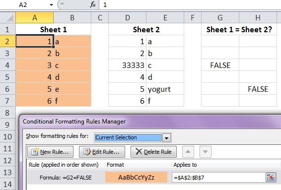
I was comparing two worksheets by creating formulas off to the side of one sheet. These returned True if the corresponding cells in the two sheets matched, False if they didn’t. I converted the Trues and Falses to values, and replaced the Trues with nothing. Then I threw some conditional formatting on the data in one of the sheets. The formatting referred to the area with empty cells and Falses. The condition was for cells offset from Falses to be shaded.

I expected a smattering of color. What I got was a solid swath of light orange. Kind of like this, but on three separate sheets:

I assumed that I’d screwed up the conditional formatting formula, a not unreasonable premise. However, after a couple of minutes I was sure I hadn’t, and it was then I realized that empty cells equate to False. I’m sure everybody else already knows this, so I figured I’d better dig a little deeper in case it comes up at a party or something.

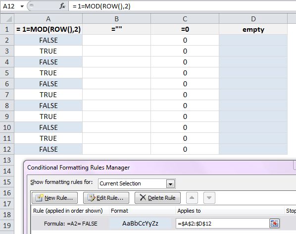
Next I checked if cells with =”” equate to False. They don’t. Neither do ones with 0, which I thought they might, since False multiplied by 1 equals 0. Here’s the visual summary, this time with a lambent blue for False.

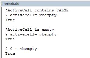
In VBA the results are similar, except that 0 = vbEmpty. I have no idea what that means. I’m pretty sure Dick had a post on this, called “testing for empty cells,” but it seems to have gone down in the great DDOE server crash of 2011.

Data Normalizer – the SQL

Posted on May 8, 2012 by Doug Glancy

In Data Normalizer I showed you how I normalize worksheet data using arrays and For/Next loops. I’ve been doing a fair amount of SQL in VBA lately, and thought I’d rewrite the code using that approach.

A little searching revealed the T-SQL/SQL Server “Unpivot” command, which normalizes your data and sets the new field names all in one swell foop. It’s not available in Access/Jet SQL though, so can’t be used on Excel. Instead, the preferred method is to use a series of Selects that pick one normalizing column at a time (along with the repeating columns) and Unions them together.

I tried ADO first, using the method of SaveCopyAs’ing the workbook-to-be-normalized in order to avoid the ADO memory leak. ADO was way slower than DAO, something like four times slower with 3000 records of 16 columns. So I went with DAO, which still takes about twice as long as the array method. Turning the ADO to DAO was easy, especially with this concise sample from XL-Dennis.

As Jeff Weir pointed out in a comment, this does require a reference (Tools>References) to the Microsoft DAO 3.5 Object Library. I’ve been switching some code over to late binding, but there doesn’t seem to be much enthusiasm for this with DAO. I’m not sure if that’s because it’s so pervasive and well-established, or for some other reason.

The core logic of the routine is pretty simple. In pseudo-English:

For each column in the columns to be normalized
Select all repeating columns
and Select (create) a new column, giving it the same name each time ("Team" in this example)
and Select the column with that team's data, giving it the same name each time ("Home Runs" in this example
and Union it to the Select statement created in the next loop iteration

Without further ado (heh heh) here’s the routine.

'Requires a reference to DAO 3.5 or later
'Arguments
'List: The range to be normalized.
'RepeatingColsCount: The number of columns, starting with the leftmost,
' whose headings remain the same.
'NormalizedColHeader: The column header for the rolled-up category.
'DataColHeader: The column header for the normalized data.
'NewWorkbook: Put the sheet with the data in a new workbook?
'
'NOTE: The data must be in a contiguous range and the
'rows that will be repeated must be to the left,
'with the rows to be normalized to the right.

Sub NormalizeList_SQL_DAO(List As Excel.Range, RepeatingColsCount As Long, _
NormalizedColHeader As String, DataColHeader As String, _
Optional NewWorkbook As Boolean = False)

Dim FirstNormalizingCol As Long, NormalizingColsCount As Long
Dim RepeatingColsHeaders As Variant, NormalizingColsHeaders As Variant
Dim RepeatingColsIndex As Long, NormalizingColsIndex As Long
Dim wbSource As Excel.Workbook, wbTarget As Excel.Workbook
Dim wsTarget As Excel.Worksheet

Dim daoWorkSpace As DAO.Workspace
Dim daoWorkbook As DAO.Database
Dim daoRecordset As DAO.Recordset
Dim strSql As String
Dim strExtendedProperties As String

With List
'If the normalized list won't fit, you must quit.
If .Rows.Count * (.Columns.Count - RepeatingColsCount) > .Parent.Rows.Count Then
MsgBox "The normalized list will be too many rows.", _
vbExclamation + vbOKOnly, "Sorry"
Exit Sub
End If
'List.Parent.Parent is the lists Workbook
Set wbSource = List.Parent.Parent
'The columns to normalize must be to the right of the columns that will repeat
FirstNormalizingCol = RepeatingColsCount + 1
NormalizingColsCount = .Columns.Count - RepeatingColsCount
'Get the header names of the repeating columns
RepeatingColsHeaders = List.Cells(1).Resize(1, RepeatingColsCount).Value
'Get the header names of the normalizing columns
NormalizingColsHeaders = List.Cells(FirstNormalizingCol).Resize(1, NormalizingColsCount).Value

strSql = vbNullString
'loop through each normalizing column
For NormalizingColsIndex = 1 To NormalizingColsCount
'Create an individual Select for the normalizing column
strSql = strSql & " SELECT "
'Select all the repeating columns
For RepeatingColsIndex = 1 To RepeatingColsCount
strSql = strSql & RepeatingColsHeaders(1, RepeatingColsIndex) & ", "
Next RepeatingColsIndex
'Select the normalizing column and assign the NormalizedColHeader field name
'and select the data being counted and assign it the DataColHeader field name
strSql = strSql & "'" & NormalizingColsHeaders(1, NormalizingColsIndex) & "'" & " AS " & NormalizedColHeader & _
", " & NormalizingColsHeaders(1, NormalizingColsIndex) & " AS " & DataColHeader
strSql = strSql & " FROM [" & List.Parent.Name & _
"$" & List.Address(rowabsolute:=False, columnabsolute:=False) & "]"
If NormalizingColsIndex < NormalizingColsCount Then
'Union the Select statements created for the normalizing columns
strSql = strSql & " UNION ALL"
End If
Next NormalizingColsIndex
End With
'Set up the DAO connection
strExtendedProperties = "Excel 8.0;HDR=Yes;IMEX=1"
Set daoWorkSpace = DBEngine.Workspaces(0)
Set daoWorkbook = daoWorkSpace.OpenDatabase(wbSource.FullName, False, True, strExtendedProperties)
Set daoRecordset = daoWorkbook.OpenRecordset(strSql, dbOpenForwardOnly)

'Put the normal data in the same workbook, or a new one.
If NewWorkbook Then
Set wbTarget = Workbooks.Add
Set wsTarget = wbTarget.Worksheets(1)
Else
Set wbSource = List.Parent.Parent
With wbSource.Worksheets
Set wsTarget = .Add(after:=.Item(.Count))
End With
End If

'copy the headers and DAO recordset to the new worksheet
With wsTarget
.Cells(1, 1).Resize(1, RepeatingColsCount).Value = RepeatingColsHeaders
.Cells(1, RepeatingColsCount + 1) = NormalizedColHeader
.Cells(1, RepeatingColsCount + 2) = DataColHeader
.Cells(2, 1).CopyFromRecordset daoRecordset
End With

'clean up
daoRecordset.Close
daoWorkbook.Close
daoWorkSpace.Close
Set daoRecordset = Nothing
Set daoWorkbook = Nothing
Set daoWorkSpace = Nothing
End Sub

If you break after strSql is created, it looks like this:

SELECT League, Year, 'ATL' AS Team, ATL AS HomeRuns FROM [HR-NL$A1:R110]
UNION ALL
SELECT League, Year, 'CHC' AS Team, CHC AS HomeRuns FROM [HR-NL$A1:R110]
UNION ALL
...
SELECT League, Year, 'MIL' AS Team, MIL AS HomeRuns FROM [HR-NL$A1:R110]

Call it like this:

NormalizeList_SQL_DAO ActiveSheet.UsedRange, 2, "Team", "HomeRuns", False

One pitfall of this SQL version is the mixed data-type issue with the Excel ISAM driver. In this example it converts all the home run counts from numbers to text because of the blanks in the data.

All in all, I think the array approach is better than SQL for this use. The core skill of creating SQL in VBA is a valuable one though, and one I’m glad to be developing.

I updated the Data Normalizer .xls to include this code.

Create Pivot Table Named Ranges

Posted on April 25, 2012 by Doug Glancy

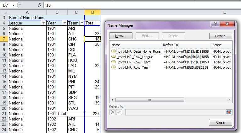
I need to calculate percentiles from subsets of data in a pivot table. In order to refer to pivot table fields, it sure would be nice if they had dynamic named ranges. So I wrote some code to create pivot table named ranges.

Programming pivot tables is fun. The extensive object model is a VBA wonderland with treats around every turn. There are great web sites out there with excellent pivot table coding samples – Contextures leaps to mind. In terms of identifying PivotFields, DataFields and other pivot table ranges, Jon Peltier wrote a superb post in 2009 that’s still generating discussion.

My code is pretty simple. It cycles through the data fields, and any other visible fields, in the specified pivot table and adds a named range for each one to the pivot table’s worksheet:

Sub RefreshPivotNamedRanges(pvt As Excel.PivotTable)
Dim ws As Excel.Worksheet
Dim pvtField As Excel.PivotField
Dim FieldType As String

With pvt
Set ws = .Parent
ClearOldNames ws, pvt
For Each pvtField In .DataFields
AddNamedRange ws, pvt.Name, "Data", pvtField.SourceName, pvtField.DataRange.Address
Next pvtField
For Each pvtField In .PivotFields
Select Case pvtField.Orientation
Case xlHidden
GoTo next_one
Case xlPageField
FieldType = "Page"
Case xlDataField
FieldType = "Data"
Case xlRowField
FieldType = "Row"
Case xlColumnField
FieldType = "Col"
End Select
AddNamedRange ws, pvt.Name, FieldType, pvtField.Name, pvtField.DataRange.Address
next_one:
Next pvtField
End With
End Sub

The PivotField.Orientation property has five enumerated constants that tell you what type of field it is – xlDataField, xlRowField, etc. The For/Next loop skips over the ones that come up xlHidden and processes the rest. Strangely, even though there’s a xlDataField type, and even though I can refer to pvt.PivotFields(“Sum of Home Runs”), the data fields don’t actually show up when cycling through the PivotFields. Instead, to get those fields the code first cycles through the pivot table’s DataFields collection.

When calling the AddNamedRange routine for a DataField, the codes passes its SourceName, not the Name. So in this example, the new name will include “Home Runs,” not “Sum of Home Runs.” You may want to pass the Name instead.

This next routine does what it says and clears out the previous range names associated with the pivot table. It’s not fool-proof. For example, if the pivot table name was changed, it won’t find the range names. I should probably use the pivot table’s Tag property to store names that won’t get changed:

Sub ClearOldNames(ws As Excel.Worksheet, pvt As Excel.PivotTable)
Dim nm As Excel.Name

For Each nm In ws.Names
If InStr(nm.Name, "!_" & pvt.Name) > 0 Then
nm.Delete
End If
Next nm
End Sub

The routine below adds the worksheet-level names to the pivot table’s sheet. It calls a function that replaces spaces and other characters that aren’t allowed in range names (code at the end of the post). It also adds a “_” at the beginning of the name to hopefully avoid illegal names like “A1”:

Sub AddNamedRange(ByRef ws As Excel.Worksheet, ByVal PivotName As String, ByVal FieldType As String, ByVal PivotFieldName As String, ByVal PivotFieldAddress As String)
Dim CleanedRangeName As String

CleanedRangeName = "_" & GetCleanedRangeName(PivotName & "_" & FieldType & "_" & PivotFieldName, "_")
ws.Names.Add Name:=CleanedRangeName, RefersTo:="=" & PivotFieldAddress & ""
End Sub

To automate this stuff, put the code in a regular module and call RefreshPivotNamedRanges from a PivotTableUpdate event. The names will be regenerated each time the pivot table is refreshed, either manually or when you drag a field, or however.

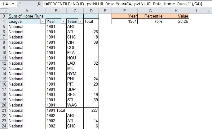
So now my Percentile array formula can find the value for the selected year and percentile:

Here’s the code to get the legal range names. You’ll need to set a reference to Microsoft VBScript Regular Expressions (at least if you’re an early binder):

Function GetCleanedRangeName(RangeName As String, SpaceReplacement As String) As String
Dim NewName As String

'the "" character escapes the Regex "reserved" characters
'x22 is double-quote
NewName = Regex_Replace(RangeName, "[\\\^\|\[\]\$\{\}\-x22/`~!@#%&=;:<>]", "", False)
'get rid of multiple contiguous spaces
NewName = Application.WorksheetFunction.Trim(NewName)
'255 is the length limit for a legal name
NewName = Left(Replace(NewName, " ", SpaceReplacement), 255)
GetCleanedRangeName = NewName
End Function

Function Regex_Replace(OriginalString As String, Pattern As String, Replacement, varIgnoreCase As Boolean) As String
' Function matches pattern, returns true or false
' varIgnoreCase must be TRUE (match is case insensitive) or FALSE (match is case sensitive)
' Use this string to replace double-quoted substrings - """[^""\r\n]*"""
Dim objRegExp As VBScript_RegExp_55.RegExp

Set objRegExp = New VBScript_RegExp_55.RegExp
With objRegExp
.Pattern = Pattern
.IgnoreCase = varIgnoreCase
.Global = True
End With
Regex_Replace = objRegExp.Replace(OriginalString, Replacement)
Set objRegExp = Nothing
End Function

This has undergone a massive .5 days of testing, so I can guarantee there’s glitches. But if you’d like to give it a spin, here you go. It’s an Excel 2007/10 file as earlier versions don’t support the “Repeat All Item Labels” pivot setting that I rely on for the Percentile array formula. Other than that, it works just as well in Excel 2003.

Prompt to Save Addins

Posted on April 18, 2012 by Doug Glancy

I’m pretty good about saving my work, and probably hit Ctrl-S a couple hundred times a day. And of course, as long as things don’t crash, Excel makes it hard to lose your work. One exception is addins, which don’t trigger a save prompt when you close them after making changes, at least when the IsAddin property is True. So I have a routine in my most-used addins that reminds me to save them. But I don’t have it in all of them. The other day this bit me, and I lost 10 minutes of work on an xlam. I decided to generalize my prompt to save addins and put it in an application-level event in my main utility addin. (These decisions come easy; what’s more fun than building a new tool?) This way I’m prompted to save any time I close an addin that I’ve changed.

If you’ve never used application-level events, Chip Pearson’s site has some good information. Okay, here’s how you can add this code to your favorite utility addin (personal.xls will do nicely).

Create a Class called “clsApplication” and paste this code into it:

Public WithEvents app As Excel.Application

Private Sub App_WorkbookBeforeClose(ByVal wb As Workbook, Cancel As Boolean)
If wb.IsAddin And Not wb.Saved Then
If MsgBox(wb.Name & "Addin" & vbCrLf & "is unsaved. Save?", _
vbExclamation + vbYesNo, "Unsaved Addin") = vbYes Then
If ExcelInstanceCount > 1 Then
MsgBox "More than one Excel instance running." & vbCrLf & _
"Save cancelled", _
vbInformation, "Sorry"
Exit Sub
Else
wb.Save
End If
End If
End If
End Sub

Create a global variable to hold the class instance. At the top of a regular code module (before any procedures) put this line:

Public cApplication As clsApplication

(I like to put all my global variables like the one above in a single module, called modGlobals.)

In the ThisWorkbook WorkbookOpen event for your utility addin, put this code:

Set cApplication = New clsApplication
Set cApplication.app = Excel.Application

One problem is that when an addin is saved with more than one instance of Excel open, it gets saved to a new location (maybe the folder of ActiveWorkbook?). So I added code to the BeforeClose event to cancel the save if that’s true. Here’s the function that does the checking:

Function GetExcelInstanceCount() As Long
Dim hwnd As Long
Dim i As Long
Do
hwnd = FindWindowEx(0&, hwnd, "XLMAIN", vbNullString)
i = i + 1
Loop Until hwnd = 0
GetExcelInstanceCount = i - 1
End Function

One last thing to do is add code to my global error handler that re-instantiates the cApplication.Class and its App property if they’ve gotten lost, which can easily happen during debugging.

Solving the NPR Sunday Puzzle – #3

Posted on April 12, 2012 by Doug Glancy

Every time I hear Will Shortz say “name a country of the world” my heart beats a little faster, cause I know there’s probably an array-formula post in it. This week was no exception:

“Name an article of clothing that contains three consecutive letters of the alphabet consecutively in the word. For example, “canopy” contains the consecutive letters N-O-P. This article of clothing is often worn in a country whose name also contains three consecutive letters of the alphabet together. What is the clothing article, and what is the country?”

This spreadsheet is live. Double-clicking in a cell in the 2nd column shows the formula. You can then drag the lower-right fill handle to see the whole gnarly thing.

Countries are a lot more list-friendly, so I solved that part first. There are two types of solutions above: an array formula in the 2nd column, and a conditional formatting solution in the 3rd to 40-somethingth column. The 2nd solution is the way I’d do it for serious work, but the array formula is more fun:

=IFERROR(
MID(A4,MIN(IF(
CODE(MID(LOWER($A4),ROW(INDIRECT("1:"& LEN($A4)-2)),1))+1=
CODE(MID(LOWER($A4),ROW(INDIRECT("2:"& LEN($A4)-1)),1)),
IF(CODE(MID(LOWER($A4),ROW(INDIRECT("1:"& LEN($A4)-2)),1))+2=
CODE(MID(LOWER($A4),ROW(INDIRECT("3:"& LEN($A4))),1)),
ROW(INDIRECT("1:"& LEN($A4)-2))))),3),
"")

This formula says to compare every letter in the country name to the next two letters. If the numeric code for a letter is one less than the letter after it, and two less than the letter after that, return those three letters. The reason the 2nd column is mostly blank is because surprisingly few country names have three consecutive letters. (Or my formula sucks.)

Here’s how it works. Let’s assume the formula refers to Albania, the 3rd country in the list:

LEN returns the length of the country’s name.

INDIRECT(“1:”& LEN($A4)-2) evaluates to (1:5).

ROW(INDIRECT(“1:”& LEN($A4)-2)) evaluates to {1;2;3;4;5}. This tells the array formula which characters in “Albania” to evaluate against their respective two next characters. Using ROW this way is very handy in array formulas.

CODE(MID(LOWER($A4),ROW(INDIRECT(“1:”& LEN($A4)-2)),1)) resolves to {97;108;98;97;110}. In other words, the numeric values of the first five letters of Albania are 97, 108, etc. CODE is the function that returns the values. LOWER converts each letter to lower case, otherwise, for example, a lowercase “b” wouldn’t be seen as following an uppercase “A”. The MID piece tells the array formula to parse each of the first 5 letters in the word.

Okay, now we’re getting close. This bit:
CODE(MID(LOWER($A4),ROW(INDIRECT(“1:”& LEN($A4)-2)),1))+1=
CODE(MID(LOWER($A4),ROW(INDIRECT(“2:”& LEN($A4)-1)),1)) resolves to
{98;109;99;98;111}={108;98;97;110;105}, which in turn resolves to {FALSE;FALSE;FALSE;FALSE;FALSE}. In other words, one added to the code for the first five letters in “Albania” doesn’t ever equal the code for their respective next letters. So there’s not even two consecutive letters. What a country! The next two lines in the formula repeat the comparison, this time with the 2nd through 7th letters.

The 2nd line, which starts with MID, and the 2nd to last line say that if the whole mess is true, return the three letters that start at that position.

The IFERROR function at the beginning and the last line simply say that if the formula errors (doesn’t find three consecutive letters) put a blank in the cell. IFERROR is available in Excel 2007 and 2010. I like it very much as they keep formulas like this from being twice as ridiculously long.

Much of the evaluation above was done using the F9 key. Selecting part of a formula and then pressing F9 evaluates that piece of the formula, a very useful feature.

There are only two countries that meet the criteria, Afghanistan and Tuvalu. I figured it was probably the former and soon enough realized the article of clothing was “hijab.”

If you’ve made it this far, thanks! Oh yeah, the multiple cell and conditional formatting way works similarly to the array formula, only by breaking it up it’s a lot easier.

If anybody has a better array formula, please share.

Copy Table Data While Not Breaking References

Posted on April 5, 2012 by Doug Glancy

I’ve mentioned before I’m a big fan of tables in Excel 2010. One way I use them is in models, where each table represents a different scenario. The models let users create new scenarios, based either on an existing one or a blank template. Each version is stored in a table in its own worksheet. These tables always have the same fields (columns) but the values in the variable fields are different. The number of rows can differ from table to table.

I often want to copy, in VBA, the contents from a “source” to a “target” table. If I just copy the whole thing, the target table will be overwritten and renamed – something like “tblSource1” (adding a “1” to the source table name). That breaks any formulas referring to “tblTarget.” They’ll show a #REF error because they can’t find “tblTarget.” So I need code that copies the table data from tblSource to tblTarget without completely replacing tblTarget.

I’ve been writing code on a case-by-case basis, but thought that I’d generalize it a bit more. In addition to keeping the table’s identity intact, it should copy the source’s totals row if there is one, and turn off the target’s total row if there isn’t. The number of rows should increase or decrease to match the source. And, although I’ve only ever copied tables as values, I want the option to copy formulas.

I thought about dealing with a different number of columns but, at least in my uses so far, that shouldn’t happen. If I ever do try to accommodate models with changing numbers of fields, I think I’d do some testing before ever calling this code, and adjust the headers in another procedure.

So here’s what I came up with:

Sub CopyTableData(loSource As Excel.ListObject, loTarget As Excel.ListObject, Optional CopyFormulas As Boolean = False)
Dim FormulaCells As Excel.Range

With loTarget
If .DataBodyRange.Rows.Count <> loSource.DataBodyRange.Rows.Count Then
'have to clear target otherwise old table content may be outside new table
.DataBodyRange.Cells.Clear
'set target rows count to source rows count
.Resize .Range.Cells(1).Resize(loSource.HeaderRowRange.Rows.Count + _
loSource.DataBodyRange.Rows.Count, loSource.Range.Columns.Count)
End If
loSource.DataBodyRange.Copy Destination:=.DataBodyRange.Cells(1)
If CopyFormulas Then
On Error Resume Next
'any formulas?
Set FormulaCells = .DataBodyRange.SpecialCells(xlCellTypeFormulas)
On Error GoTo 0
'if yes, then replace any references to source table with target
If Not FormulaCells Is Nothing Then
FormulaCells.Replace what:=loSource.Name, replacement:=.Name, lookat:=xlPart
End If
Else
.DataBodyRange.Value2 = .DataBodyRange.Value2
End If

'turn target Totals row on or off to match Source
If loSource.ShowTotals Then
.ShowTotals = True
loSource.TotalsRowRange.Copy Destination:=.TotalsRowRange
Else
.ShowTotals = False
End If
End With

End Sub

One thing I learned is that there are two Resizes in a table (listobject). The first type, the Range property, was familiar, e.g.,

Range("A1").Resize(20,1)

… which yields a range object whose address is A1:A20.

The second is the Listobject.Resize method, which allows you to modify a table’s range, e.g.,

loTarget.Resize(Range("A1:F20")

which will change loTarget’s range to A1:F20.

Both of these types of Resizes are used in the code above, in the same line, happily enough.

Data Normalizer

Posted on March 28, 2012 by Doug Glancy

Sometimes I get data like this…

that needs to be like this…

The goal here is to roll up all the home runs into one, much longer, column. The data will then be pivot-worthy.

Generally, I need to keep one or more leftmost column headers, in this case “League” and “Year.” I need a new column to describe the rolled-up category (“Team”) and one for the data itself (“Home Runs”). I’ve written code a couple of times to handle specific cases and thought I’d try to generalize it. Here’s the result:

'Arguments
'List: The range to be normalized.
'RepeatingColsCount: The number of columns, starting with the leftmost,
' whose headings remain the same.
'NormalizedColHeader: The column header for the rolled-up category.
'DataColHeader: The column header for the normalized data.
'NewWorkbook: Put the sheet with the data in a new workbook?
'
'NOTE: The data must be in a contiguous range and the
'rows that will be repeated must be to the left,
'with the rows to be normalized to the right.

Sub NormalizeList(List As Excel.Range, RepeatingColsCount As Long, _
NormalizedColHeader As String, DataColHeader As String, _
Optional NewWorkbook As Boolean = False)

Dim FirstNormalizingCol As Long, NormalizingColsCount As Long
Dim ColsToRepeat As Excel.Range, ColsToNormalize As Excel.Range
Dim NormalizedRowsCount As Long
Dim RepeatingList() As String
Dim NormalizedList() As Variant
Dim ListIndex As Long, i As Long, j As Long
Dim wbSource As Excel.Workbook, wbTarget As Excel.Workbook
Dim wsTarget As Excel.Worksheet

With List
'If the normalized list won't fit, you must quit.
If .Rows.Count * (.Columns.Count - RepeatingColsCount) > .Parent.Rows.Count Then
MsgBox "The normalized list will be too many rows.", _
vbExclamation + vbOKOnly, "Sorry"
Exit Sub
End If

'You have the range to be normalized and the count of leftmost rows to be repeated.
'This section uses those arguments to set the two ranges to parse
'and the two corresponding arrays to fill
FirstNormalizingCol = RepeatingColsCount + 1
NormalizingColsCount = .Columns.Count - RepeatingColsCount
Set ColsToRepeat = .Cells(1).Resize(.Rows.Count, RepeatingColsCount)
Set ColsToNormalize = .Cells(1, FirstNormalizingCol).Resize(.Rows.Count, NormalizingColsCount)
NormalizedRowsCount = ColsToNormalize.Columns.Count * .Rows.Count
ReDim RepeatingList(1 To NormalizedRowsCount, 1 To RepeatingColsCount)
ReDim NormalizedList(1 To NormalizedRowsCount, 1 To 2)
End With

'Fill in every i elements of the repeating array with the repeating row labels.
For i = 1 To NormalizedRowsCount Step NormalizingColsCount
ListIndex = ListIndex + 1
For j = 1 To RepeatingColsCount
RepeatingList(i, j) = List.Cells(ListIndex, j).Value2
Next j
Next i

'We stepped over most rows above, so fill in other repeating array elements.
For i = 1 To NormalizedRowsCount
For j = 1 To RepeatingColsCount
If RepeatingList(i, j) = "" Then
RepeatingList(i, j) = RepeatingList(i - 1, j)
End If
Next j
Next i

'Fill in each element of the first dimension of the normalizing array
'with the former column header (which is now another row label) and the data.
With ColsToNormalize
For i = 1 To .Rows.Count
For j = 1 To .Columns.Count
NormalizedList(((i - 1) * NormalizingColsCount) + j, 1) = .Cells(1, j)
NormalizedList(((i - 1) * NormalizingColsCount) + j, 2) = .Cells(i, j)
Next j
Next i
End With

'Put the normal data in the same workbook, or a new one.
If NewWorkbook Then
Set wbTarget = Workbooks.Add
Set wsTarget = wbTarget.Worksheets(1)
Else
Set wbSource = List.Parent.Parent
With wbSource.Worksheets
Set wsTarget = .Add(after:=.Item(.Count))
End With
End If

With wsTarget
'Put the data from the two arrays in the new worksheet.
.Range("A1").Resize(NormalizedRowsCount, RepeatingColsCount) = RepeatingList
.Cells(1, FirstNormalizingCol).Resize(NormalizedRowsCount, 2) = NormalizedList

'At this point there will be repeated header rows, so delete all but one.
.Range("1:" & NormalizingColsCount - 1).EntireRow.Delete

'Add the headers for the new label column and the data column.
.Cells(1, FirstNormalizingCol).Value = NormalizedColHeader
.Cells(1, FirstNormalizingCol + 1).Value = DataColHeader
End With
End Sub

You’d call it like this:

Sub TestIt()
NormalizeList ActiveSheet.UsedRange, 2, "Team", "Home Runs", False
End Sub

It runs pretty fast. The sample sheet above – 109 years of data by 16 teams – completes instantly. 3,000 rows completes in a couple of seconds.

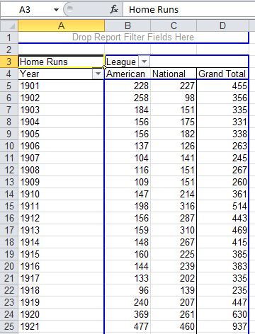
If I also run the routine on some American League data and put all the new rows in one sheet (with the same column headers) I can generate a pivot table that looks like this, which I couldn’t have done with the original data:

You can download a zip file with a .xls workbook that contains the data and code. Just click on the “normalize” button.

Anything

Posted on March 23, 2012 by Doug Glancy

I think about this blog a lot. I’m always pondering the next post, a challenge given the multitude of great ones that have gone before. I’ve tinkered with WordPress quite a bit, which is fun. Using it inspired me to create this gravatar …

… which I like to call the “smiling sigma.”

And I check my stats (such as they are) a lot. One of my favorites is the list of search terms bringing people to this site.

Search Terms

The two most common have to do with pivot tables and conditional formatting. After that there are a few concerning the NPR Sunday Puzzle, and I’m proud to note that when I google “NPR Sunday Puzzle,” this site is right up there in the results.

Here’s some of my favorites:

“word puzzle first letter hero villain world capital blog” – definitely an NPR Sunday Puzzle solver

“toolbar lengkap excel 2003” – I understand that “lengkap” is Indonesian for “complete”

“goofy code” – I rank very high in the results on this, hopefully only because there’s a post here with that name

My Second Most Favorite Search Term

“sum buddy i use to no” – Now there’s a person after my own heart! What were they looking for? And how do you “use somebody to no” anyways? It sounds handy.

Sadly, I’ll never no.

My Most Favorite Search Term

“Anything”

Yup, according to AwStats, somebody googled “anything” and ended up here. I’m not completely convinced this happened, but it’s there on my screen, so I’m going with it.

A Flexible VBA Chooser Form

Posted on March 20, 2012 by Doug Glancy

Fairly often in VBA code I need to offer the user a list and have them make a choice, like picking which open workbook to do something to. I created a function and a userform to handle these situations. (Around the house, I call the form “ChooserForm” but it’s given name is “frmChooser.”) The function takes an array of choices and a caption as its arguments. The function loads frmChooser and passes it the string array and the caption. When the user makes a choice and clicks OK the function returns the choice to the calling routine.

Let’s look at how it works, starting from the inside out (by which I mean with the userform):

The frmChooser UserForm

Private mboolClosedWithOk As Boolean
Private mChoiceList() As String

Public Property Let ChoiceList(PassedList() As String)
mChoiceList() = PassedList()
End Property

Private Sub UserForm_Activate()
With Me.cboChooser
.List = mChoiceList()
.ListIndex = 0
End With
End Sub

Public Property Get ChoiceValue() As String
ChoiceValue = Me.cboChooser.Value
End Property

Private Sub cmdOk_Click()
mboolClosedWithOk = True
Me.Hide
End Sub

Public Property Get ClosedWithOk() As Boolean
ClosedWithOk = mboolClosedWithOk
End Property

Private Sub cmdCancel_Click()
mboolClosedWithOk = False
Me.Hide
End Sub

Private Sub UserForm_QueryClose(Cancel As Integer, CloseMode As Integer)
'in case the user clicked the "X"
If CloseMode = vbFormControlMenu Then
Cancel = True
cmdCancel_Click
End If
End Sub

The form has three custom properties. The first, Let ChoiceList, assigns the array of choices to the form’s module-level variable, mChoiceList(). On form activation the combobox cboChooser’s list is filled with the mChoiceList array.

The second property, Get ChoiceValue, is the currently selected value of the combobox. The function will “get” this, after the OK button is clicked, to determine the user’s choice.

The third property, Get ClosedWithOk tells the calling function whether the user hit the OK button. If it’s True then the function will do its processing. If it’s false, then the user hit the Cancel button or the “X,” and we’ll skip the processing.

The Function code

Function GetChoiceFromChooserForm(strChoices() As String, strCaption As String) As String
Dim ufChooser As frmChooser
Dim strChoicesToPass() As String

'why is this necessary?
ReDim strChoicesToPass(LBound(strChoices) To UBound(strChoices))
strChoicesToPass() = strChoices()
Set ufChooser = New frmChooser
With ufChooser
.Caption = strCaption
.ChoiceList = strChoicesToPass
.Show
If .ClosedWithOk Then
GetChoiceFromChooserForm = .ChoiceValue
End If
Unload ufChooser
End With
End Function

The function creates an instance of frmChooser, called “ufChooser,” passes the Caption and ChoiceList properties and shows the form. After the .Show command, processing passes into the form and the code shown in the previous section. Processing returns to the function when the form is hidden, by either the OK or Cancel button’s click event. The function then checks the form’s ClosedWithOK property. If it’s true the function returns the form’s ChoiceValue property – the value selected in the combobox – to the calling routine.

You may have noticed the question “why is this necessary?” I can’t just pass strChoices() straight into the frmChooser instance. It causes a runtime “internal error.” Instead I have to declare a second string array strChoicesToPass() and copy the first array to it. If anybody can explain why, please share! (I think I could pass a variant straight through, but I don’t.)

The general form of this function’s code, and that of the userform, is from the venerable Professional Excel Development.

Using the Function

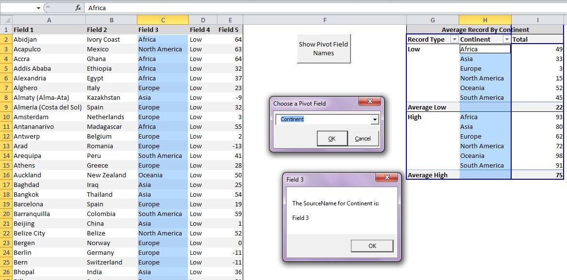
Now that we’ve got the function and the form, let’s choose something! I’ve got some code below that lists all the visible fields in a pivot table. When one is picked, the data range for the field is highlighted, along with the source column in the table, and the fields source name is displayed:

Sub ShowPivotFieldInfo()
Dim pvt As Excel.PivotTable
Dim lo As Excel.ListObject
Dim StartingCell As Excel.Range
Dim i As Long
Dim PivotFieldNames() As String
Dim pvtField As Excel.PivotField
Dim ChosenName As String

Set pvt = ActiveSheet.PivotTables("pvtRecordTemps")
Set lo = ActiveSheet.ListObjects("tblRecordTemps")
Set StartingCell = ActiveCell
With pvt
ReDim PivotFieldNames(1 To .VisibleFields.Count) As String
For i = 1 To .VisibleFields.Count
PivotFieldNames(i) = .VisibleFields(i).Name
Next i
ChosenName = GetChoiceFromChooserForm(PivotFieldNames, "Choose a Pivot Field")
If ChosenName = vbNullString Then
Exit Sub
End If
Set pvtField = .PivotFields(ChosenName)
With pvtField
Union(.DataRange, lo.ListColumns(.SourceName).DataBodyRange).Select
MsgBox Title:=.SourceName, _
Prompt:="The SourceName for " & ChosenName & " is:" & vbCrLf & vbCrLf & .SourceName
End With
StartingCell.Select
End With
End Sub

This type of code can be useful when the PivotField names have been changed drastically from their underlying SourceNames, especially if the SourceNames are cryptic, similar, and there’s lots of them. In the picture below the SourceNames in the table were “Field 1”, “Field 2”, etc., but were changed to meaningful names like “Continent” in the pivot table.

Here’s the sample workbook for your downloading pleasure.