The Best Min Function, I Think

A few weeks ago I wrote a Min array function to determine the minimum of a subset of items in a table. It was not the best Min function, in fact it didn’t work. I’d based it on the Max function I’d written moments earlier – a rookie mistake – and it resulted in zero when it shouldn’t have. I fixed it, but the fix was ugly. Then I realized I could use an If statement in an array formula, which helped a lot. Then I read this informative and lively post.

I’ll summarize what I learned, and propose my own Best Min Function, using the interactive workbook below.

The Workbook

The table on the left contains record high and low Fahrenheit temperatures from various cities around the world, listed by continent. (Column B contains the countries. You can unhide it.)

The formulas are in the table in the top right. They all look for the lowest of the record lows by continent.

Below the formulas are a couple of cells which trigger a couple of pitfalls of the Min function. Below that are text versions of the formulas.

The Formulas

The first formula, “multiplication,” is my original failure. The conditions (record type and continent) and the record lows are all multiplied:

{=MIN((tblRecLows[Record Type]="Low")*(tblRecLows[Continent]=H$1)*
(tblRecLows[Record]))}

As described in the post linked above, this only works for Min if at least one value is equal to or less than zero. Multiplying arrays of conditions like this will always yield some zeros – whenever all the conditions aren’t met – and so the minimum can never be higher than zero.

This list low temps is illustrates the problem well. For some continents the record low is negative, but for others it’s positive. You can see that this formula fails for continents where the record low is positive. For example Africa should show 30 degrees, but it shows zero.

My fix was to force all the numbers in the table to be negative, by subtracting the maximum record temperature from each number, find the minimum, and then add the maximum back. This eliminates the zero problem…

{=MIN((tblRecLows[Record Type]{="Low")*(tblRecLows[Continent]{=H$1)*
(tblRecLows[Record]-(MAX(tblRecLows[Record])+1)))+(MAX(tblRecLows[Record])+1)}

… but it’s ugly. And anyways, both multiplication versions fail if there is any stray text in your list. I noticed this because Florence had “NA’s” for both high and low records. The multiplication chokes on the text value, just as it would on 2 * “NA”, and the formula fails. You can see this by changing the “Has Text” in the “Potential Pitfalls” section to True. Both formulas yield #VALUE.

So, as faithful readers of DDOE already knew – at least if their memories are better than mine – If statements are the way to go. The “nested If” and the “Elias one-if” versions above work because they return an array filled either with temperatures that meet all the criteria, or Falses. The Min function ignores the Falses, and so returns the correct minimum.

Now for the second pitfall: Empty cells in your list are a problem because an IF statement cannot return a null. It converts blank cells to zeroes which, you guessed it, become the result of the Min function if there’s no lower number.

You can see this by changing the “Has Blanks” in the “Potential Pitfalls” section to True and following the instructions. You’ll see that the “nested if” and “Elias one-if” both fail for Africa, and will for any warm continent with a blank cell.

The proposed “Best Min” solves this problem by adding a criteria of non-blank cells. (It also eliminates the “>0” check of the multiplied conditions from Elias’s version as it seems to evaluate to the same thing.)

{MIN(IF(((tblRecLows[Record Type]="Low")*(tblRecLows[Continent]=H$1)*
(tblRecLows[Record]<>"")),tblRecLows[Record]))}

There is a runner-up at the end of the list: a GetPivotData formula looking into a pivot table, or perhaps just a pivot table itself (you’ll see it if you scroll down). It might be my first choice if if didn’t require refreshing.

One last thought

I just realized that the Max function is subject to the exact same false-zero-minimum problems if all values are equal to or below zero, the inverse of the Min issue.
Solving the NPR Sunday Puzzle – #2

This week’s NPR Sunday Puzzle was array formula nirvana.

“Take the trees hemlock, myrtle, oak and pine. Rearrange the letters in their names to get four other trees, with one letter left over. What trees are they?”

I made this workbook to solve the puzzle:

At the left is a list of trees whose names meet three criteria:

  • The name only contains letters from the four starting trees.
  • The name doesn’t contain more of any letter than are in the four starting names combined.
  • The name isn’t in the original list.

To solve the puzzle, enter TRUE next to trees to choose them. The list of letters on the right will change as you do. Letters shaded blue are still available and the number remaining is shown. If a letter is shaded orange, you’ve overused it and the “remaining” number is negative. Unshaded letters have been used perfectly.

When the number of trees selected is four and one letter is unused, you’ve solved the puzzle. Go ahead and try it! And, oh yeah, there may be something tricky about the list.

Now for the array formulas, all entered with Ctrl-Shft-Enter. There’s one in the “Used” column:

{=SUM(LEN(IF(tblTrees[Use?],tblTrees[Tree],"")))-
SUM(LEN(SUBSTITUTE(IF(tblTrees[Use?],tblTrees[Tree],""),[@[Letters To Use]],"")))}

It compares the length of the names chosen against the length of their names after removing the letter, i.e., how many times that letter is used.

To get the list of tree names my family did some brainstorming, which we augmented with a list from the web. It was sliced and diced using Text to Columns and Remove Duplicates from the Excel 2010 Data menu.

Two more array formulas winnow the list to names that meet our three criteria. They’re on the “Good Trees” tab of the workbook. The “Contains Only Valid Letters” formula determines if a name meets the first criteria:

{=MATCH(0,COUNTIF(tblLetters[Letters To Use],
MID($A2,{1,2,3,4,5,6,7,8,9,10,11,12,13,14,15},1)),0)>LEN($A2)}

This formula assumes that the longest name is 15 letters. The CountIf increments through the letters in the word, counting the occurrences of each letter in the list, which will either be one or zero. It uses Match to find the position of the first zero. If that’s greater than the number of letters in the word it passes the test.

The “Contains Less Of Each Letter Than Total” formula checks our second criteria:

{=ISERROR(MATCH(FALSE,(tblLetters[Count Of Letter]>=
(LEN(A2)-LEN(SUBSTITUTE(A2,tblLetters[Letters To Use],"")))),0))}

This also uses the trick of comparing the length of the name against its length with the character removed, to get the count of that letter in the word. It then assumes that the count of that letter overall is greater than or equal to the count in the word, for each letter in the word. If that assumption is FALSE in any letter position the word is no good.

The “Not In Original List” formula checks … you know. The last one combines the first three and if they’re all true the word makes the cut.

I’d love to hear how other people would do these tests. I’m curious too if others are using Excel to solve puzzles, NPR or otherwise. Do you have a good source of lists? I always just google around, with mixed results.

After I had done all the processing I used the workbook to get the answer. I chose three names – elm, hickory and lemon, and had a, e, k, p and t left over. Four of those letters spelled the last tree. It wasn’t on the list but I added it. You could just put it where pecan is now if you want. If you already did, then “teak” a bough. Yew should be proud.

Speaking of tree-related words, one of my favorite words is “pitch.” It’s arboreal, nautical, romantic, and so much more.

A Prefix Function to Save You From VBA Magic Numbers, Sometimes

Magic Numbers in Formulas

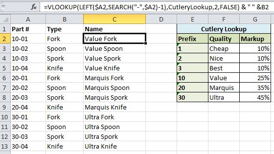
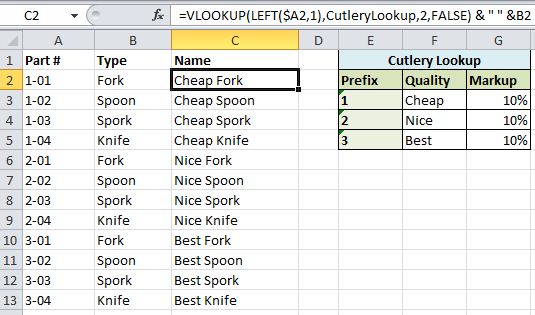
The last post referred to “magic numbers” and the pitfalls of using them in formulas. An example might be this product list, where the quality level is represented by a single digit before the dash in the part number, the “quality prefix.”

lookup formula with magic number

The formula generating the name in C2 is a simple one. It does a lookup of the quality prefix – 1, 2, or 3 – in the “Cutlery Lookup” table, yielding a quality of “Cheap,” “Nice” or “Best.” This is added to the product type, resulting in a name such as “Nice Spork.”

=VLOOKUP(LEFT($A2,1),CutleryLookup,2,FALSE) & " " &B2

One day the proprietors realize these lackluster brand names are a drag on sales. They create new codes and names for the products, adding a 0 to the quality prefix and new quality descriptions to the table. They then print up 2,000 parts lists, failing to notice that the formula is still generating the same lousy names.

new quality prefix - same names
This is due to the magic number “1” in the “VLOOKUP(LEFT($A2,1)” part. It still specifies the length of the quality prefix as 1, meaning the lookup is still seeking the prefixes 1, 2 and 3. (Admittedly, their luck was bad in choosing new codes that didn’t result in #NA and in leaving in the old ones, but they were probably forced to by other bad design practices.)

A more robust approach is to have the formula look for the dash separating the quality code from the rest of the product number, like:

=VLOOKUP(LEFT($A2,SEARCH("-",$A2)-1),CutleryLookup,2,FALSE) & " " &B2

lookup formula with calculated number

This will accommodate different length prefixes.

Magic Numbers and Prefixes in VBA

Prefixes in VBA can also lead to magic numbers. Say you have a workbook with some worksheets identified by the prefix “final” in the name. To process these sheets you might write code like:

Dim ws As Excel.Worksheet
For Each ws In ThisWorkbook.Worksheets
    If Left(ws.Name, 5) = "Final" Then
        ProcessSheet ws
    End If
Next ws

Of course, it’s always dangerous to use the word “final” in a name because nothing’s ever finished. So the next week when the “Really Final” worksheets need to be processed, you change your code to:

If Left(ws.Name, 5) = "Really Final" Then

and the Left function finds no sheet names whose first 5 letters are “Really Final.”

I’ve done something like this more than once, so I wrote a HasPrefix function to end it:

Function HasPrefix(StringToCheck, Prefix, Optional CaseSensitive As Boolean = False) As Boolean
If CaseSensitive Then
    HasPrefix = Left((StringToCheck), Len(Prefix)) = Prefix
Else
    HasPrefix = Left(LCase(StringToCheck), Len(Prefix)) = LCase(Prefix)
End If
End Function

You pass it the string to check, along with the prefix you’re checking for (and whether it’s case-sensitive if you want). It uses the length of the prefix in the Left function, so the length won’t ever be wrong.

I used this recently to check whether a workbook was located in the AppData folder in the user profile, meaning it was most likely opened from an email:

If HasPrefix(ActiveWorkbook.FullName, Environ("LOCALAPPDATA")) then

(Environ is a handy Windows function for checking on your computer’s settings and JP has an informative article on it.)

Two-dimensional Index/Match Formula with Variable-Length Lookup

When I was a housing developer I used Excel for budgets and pro formas. I wrote PPMT formulas, did lots of Goal Seeking, and never used pivot tables. Now I use them all the time, and my favorite formula is an Index/Match. It’s gotten to where I can type a fancy lookup pretty quickly, though my array formulas generally take a bit of hacking. I’m no Barry Houdini, but I do all right.

Yesterday I realized you can do a Match into an array of substrings of cell values. For example, in this baseball stats sheet (I think it’s “rhubarbs” per year) you can match against just the beginning few characters of each column heading, like “SF” or “STL.”

Here’s the formula in cell I3. Note that it’s an array formula, entered with Ctrl-Shft-Enter:

=INDEX(tblRhubarb,
MATCH($G$3,tblRhubarb[YEAR],0),
MATCH(TEXT($H$3,"0"),LEFT(tblRhubarb[#Headers],LEN($H$3)),0))
  • The first part, “INDEX(Table2”, says to index into the whole table. In other words, it’s a two-dimensional lookup.
  • The second part, “MATCH($G$3,tblRhubarb[YEAR],0),” says to look in the year column for a match to the year in G3.
  • The third part, “MATCH(TEXT($H$3,”0″),LEFT(tblRhubarb[#Headers],LEN($H$3)),0))” says to look in the column headers for the team abbreviation in H3.

I wasn’t sure that last section would work. It says to look only in the left part of each header. When you analyze this last part by highlighting it and hitting F9 it looks like…

MATCH(TEXT($H$3,"0"),{"YE","LA"," P","SF","ST"},0))

… which is pretty cool.

The final thing to mention is about this part of the formula:

LEN($H$3)

This says to look at the leftmost number of characters equal to the length of the string in H3. That’s important because not all the team abbreviations are the same length. It would be important even if they were, because you don’t want to rely on “magic numbers” in formulas or code.

If you’re interested in these types of formulas be sure to go back to the top of the post and click the barry houdini link. Not only does he have a great name, he could write a formula that would find your car keys, and it wouldn’t even have to be array-entered.

Excel Recent File Deleter

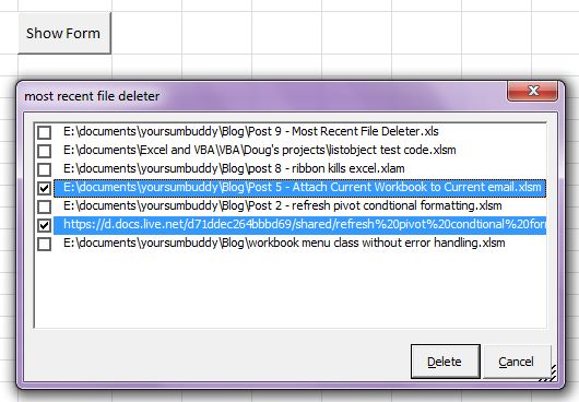
Although the downloadable file is in Excel 2003 format, I never needed one of these until Excel 2010. Now I use the recent files list a lot more, and I want to be able to tidy it up without having to right-click files one at a time. Hence the creation of this simple tool, which allows you to delete multiple entries from the list.

Recent

The form’s initialization code fills the listbox with the recent files. It sets the listbox’s style to the fabulously clunky fmListStyleOption, and MultiSelect to Extended. This means you can select multiple files using the control and shift keys. You can’t uncheck an item though, except by selecting another.

With Me.lstRecentItems
    For i = 1 To Application.RecentFiles.Count
        Me.lstRecentItems.AddItem Application.RecentFiles(i).Path
    Next i
    .ListStyle = fmListStyleOption
    'you can use ctrl and shft to select multiple files
    .MultiSelect = fmMultiSelectExtended
    .ListIndex = -1
End With

The UserForm also has code from Andy Pope for making the form resizable, which I tinkered with a bit.

The Delete button code loops backwards through the listbox, deleting the corresponding file if the item is selected. It goes backwards for the same reason you delete rows from bottom to top – otherwise the indexing gets messed up and you delete the wrong files.

Private Sub cmdDelete_Click()
Dim i As Long

With Me.lstRecentItems
    'If nothing's chosen
    If .ListIndex = -1 Then
        GoTo exit_point
    End If
    For i = .ListCount - 1 To 0 Step -1
        If .Selected(i) Then
            'List is zero-based, RecentFiles is a one-based collection
            Application.RecentFiles(i + 1).Delete
        End If
    Next i
End With
'If you're looking at the Home screen this will update it
Application.ScreenUpdating = True

exit_point:
CloseForm

End Sub

I’d like it if you could bring the “pinned” items to the top of the listbox, but I don’t see any properties or objects to control that. Recentfiles seems to be simply indexed with the most recent first.

If you play around with this and, like me, delete all the files from your list, you can fill it back up with fictitious ones.

Sub FillMostRecentList()
Dim i As Long

For i = 1 To 20
    Application.RecentFiles.Add ("c:/test" & i)
Next i
Application.ScreenUpdating = True
End Sub

Download the Recent File Deleter zip file.

A Workbook-Hooker with no Ribbon-related fatalities

I’ve been working on an addin that uses application-level events to “hook” certain “target” workbooks as they open, in order to control menus and other functionality for the target workbooks. I like this setup because the code is all in the addin, so code updates don’t bother users and they don’t have to enable macros.

The Basics

The application class is created when the addin starts, and application-level events track the opening and closing of target workbooks. When a target opens, a workbook class is instantiated. That gets added to a dictionary object that contains all currently open target workbooks. The workbook class shows the ribbon tab when the workbook is activated and hides it when the workbook is deactivated.

I had never created an addin like this using ribbon menus. Creating a new ribbon group is easy using Andy Pope’s RibbonX Visual Designer. And I added the ribbon loss-of-state insurance Ron de Bruin demonstrates. But the ribbon did cause problems when I tried to address a couple of potential usage situations.

The Tricky Parts

If the addin is not checked in the Addins dialog, I want it to behave well when a user does check it. This means that if a target workbook is already open, the menu should be shown when the addin starts. The menu should also be shown if a user opens Excel by clicking on a target workbook in Windows Explorer. I tried to set this up in the addin’s ThisWorkbook module by calling initialization code from the Addin_Install and Workbook_Open events. However, this consistently crashed Excel in these two situations. Somehow my code was colliding with the ribbon’s instantiation. I tried to solve this by delaying initialization with Application.OnTime. This worked for the addin-activation scenario, but not for the Windows Explorer one. My code was somehow trying to run at the same time, or before, the ribbon’s code.

Finally, finally, it hit me that the solution was to call all my initialization code from the Ribbon_OnLoad event. That seems to have fixed the problem, and now there’s no code in the addin’s ThisWorbook module at all.

One other thing I learned was that an application-level Workbook_Open event is fired when you attempt to re-open an open workbook, either from Windows Explorer or in Excel. This could lead to trying to re-add a workbook to the Dictionary if the user accidentally tried to open an already open workbook, so I just re-load the dictionary each time.

The Code

(You can also follow the link at the end of this post to downdoad the addin and two targets.)

Here’s the Application Class module, called clsApplication. Along with hooking target workbooks when they open, it removes them from the collection when they’re closed, using the application’s BeforeClose and Deactivate events.

Public WithEvents App As Excel.Application
Private mboolWbClosing As Boolean

Private Sub App_WorkbookOpen(ByVal wb As Workbook)
If WbIsTargetWorkbook(wb) Then
    FillDictionary
End If
End Sub

Private Sub App_WorkbookBeforeClose(ByVal wb As Workbook, Cancel As Boolean)
'The last close might have been cancelled
mboolWbClosing = False
If gdicTesterWorkbooks.Exists(wb.Name) Then
    'It might be closing, but the close might be cancelled
    mboolWbClosing = True
End If
End Sub

Private Sub App_WorkbookDeactivate(ByVal wb As Workbook)

If mboolWbClosing Then
'Okay, it's really closing
    If gdicTesterWorkbooks.Exists(wb.Name) Then
        gdicTesterWorkbooks.Remove wb.Name
    End If
    mboolWbClosing = False
End If
End Sub

This is the clsTargetWorkbook class.

Public WithEvents wb As Excel.Workbook

Private Sub Class_Initialize()
SetRibbonVisibility True
End Sub

Sub wb_Activate()
SetRibbonVisibility True
End Sub

Sub wb_Deactivate()
SetRibbonVisibility False
End Sub

Last is a module with the remaining code. It includes global variables to track the comings and goings of the ribbon, along with the class and dictionary declarations. Below that is the section that helps retrieve the ribbon reference should it be lost, followed by the subs for the actual ribbon events. Finally, there’s routines to manage the application class and dictionary, test for target workbooks, and show and hide the ribbon. (It probably goes without saying that the real version doesn’t use workbook names to test for target workbooks.)

'thanks to Rory Archibald and Ron de Bruin for Ribbon
'loss-of-state prevention code
'http://www.rondebruin.nl/ribbonstate.htm

Public gRibbon As IRibbonUI
Public cApplication As clsApplication
Public cTargetWorkbook As clsTargetWorkbook
Public gdicTesterWorkbooks As Object
Public gboolShowRibbonTab As Boolean

#If VBA7 Then
    Public Declare PtrSafe Sub CopyMemory Lib "kernel32" Alias "RtlMoveMemory" (ByRef destination As Any, ByRef source As Any, ByVal length As Long)
#Else
    Public Declare Sub CopyMemory Lib "kernel32" Alias "RtlMoveMemory" (ByRef destination As Any, ByRef source As Any, ByVal length As Long)
#End If

#If VBA7 Then
    Function GetRibbon(ByVal lRibbonPointer As LongPtr) As Object
#Else
    Function GetRibbon(ByVal lRibbonPointer As Long) As Object
#End If

Dim objRibbon As Object
CopyMemory objRibbon, lRibbonPointer, LenB(lRibbonPointer)
Set GetRibbon = objRibbon
Set objRibbon = Nothing
End Function

Public Sub Ribbon_onLoad(ribbon As IRibbonUI)
Set gRibbon = ribbon
ThisWorkbook.Names.Add Name:="RibbonPointer", RefersTo:=ObjPtr(ribbon)
ThisWorkbook.Saved = True

'only do our initialization after the ribbon's

InitializeGlobals
FillDictionary
End Sub

Sub InvalidateRibbon()
If gRibbon Is Nothing Then
    Set gRibbon = GetRibbon(Replace(ThisWorkbook.Names("RibbonPointer").RefersTo, "=", ""))
End If
gRibbon.Invalidate
End Sub

Public Sub grpRibbonTester_getVisible(control As IRibbonControl, ByRef returnedVal)
returnedVal = gboolShowRibbonTab
End Sub

Public Sub cmdTester_onAction(control As IRibbonControl)
MsgBox "testing"
End Sub

Sub InitializeGlobals()
Set cApplication = New clsApplication
Set cApplication.App = Application
Set gdicTesterWorkbooks = CreateObject("Scripting.Dictionary")
End Sub

Sub FillDictionary()
Dim wb As Excel.Workbook
Dim cTargetWorkbook As clsTargetWorkbook

Set gdicTesterWorkbooks = Nothing
Set gdicTesterWorkbooks = CreateObject("Scripting.Dictionary")
For Each wb In Workbooks
    If WbIsTargetWorkbook(wb) Then
        Set cTargetWorkbook = New clsTargetWorkbook
        Set cTargetWorkbook.wb = wb
        gdicTesterWorkbooks.Add cTargetWorkbook.wb.Name, cTargetWorkbook
    End If
Next wb
End Sub

Function WbIsTargetWorkbook(wb As Excel.Workbook)
If wb.Name = "Target1.xlsx" Or wb.Name = "Target2.xlsx" Then
    WbIsTargetWorkbook = True
End If
End Function

Sub SetRibbonVisibility(boolRibbonVisible As Boolean)
gboolShowRibbonTab = boolRibbonVisible
InvalidateRibbon
End Sub

The Download, Should You So Desire

A zipped file with the addin, and two target workbooks. Install the addin, open the workbooks, or vice-versa.

Percent of True Items in a Pivot Table Field

Sometimes you may want to use a pivot table to summarize data whose values are either true or false. For example, whether congressional representatives have law degrees, whether cities have chlorinated water supplies, or whether students are taking classes at the honors level. I’m thinking of traits which exist not in opposition to another trait, e.g., blue eyes versus brown, but, in isolation, e.g., “has brown eyes.” In many cases, such as pulling from a database, these types of items are only filled if they’re true, otherwise they are left blank.

While struggling to summarize some data like this in a single column of a pivot table, I had the following realization:

The percentage of True items in a list is the average of zeros and ones, where True is represented by 1 and False by 0.

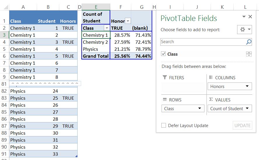
For example, assume you have a list of students in different classes, some of whom are taking the class at the honors level. This is indicated in an”Honors” column that’s either marked True or left blank. (Note that the following would work exactly the same if the blanks were instead marked False.)

The Clunky Way

To show the percent at the honors level, you could pivot on the Honors column as it is, but you’d have to show both the True and blank values, as in the pivot table below:

Pivot True and False

In this pivot table, the Values field is Students, “Summarize Values By” is set to “Count” and “Show Values As” is set to “% of Row Total”.

With this setup you’re stuck with using two pivot table columns. If you uncheck “(blank)” in the Honors dropdown, the pivot table reports 100% for every class, since it’s now filtered to only the True items.

The Un-Clunky Way

So instead let’s add a helper column to our data. I called it “Honors for Average” in the picture below. It just multiplies the adjacent Honors column cell by one, resulting in either 0 or 1.

helper column added

We can now pivot on the Honors for Average column. In the pivot table below, Class is in the Row area and the Value field is Honors for Average. “Show Values As” is set to the default of “No Calculation” and, most important, “Summarize Values By” is set to “Average.”

pivot-True only

Then, to finish it up, I changed the title to something more meaningful.

title changed

I think this is a much clearer and more concise way to represent this type of data.

Solving the NPR Sunday Puzzle

The yoursumbuddy official smartphone has two alarms. One wakes me up at the reasonable hour of 6:23, and one goes off at 9:35 every Sunday with a reminder that NPR’s Sunday Puzzle starts in three minutes. Last Sunday’s lent itself nicely to some Excel fun:

“Name two fictional characters – the first one good, the second one bad. Each is a one-word name. Drop the last letter of the name of the first character. Read the remaining letters in order from left to right. The result will be a world capital. What is it?”

To solve this, I wanted a list of villains and another of world capitals.

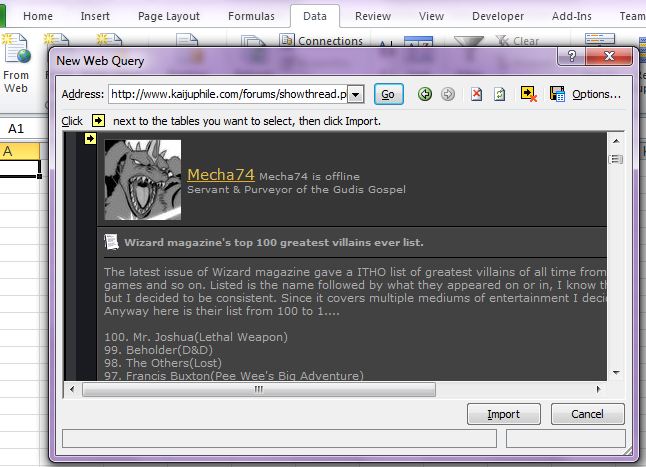
I recently realized that Excel’s Data > From Web feature is easier than copying stuff straight from the web. A lot of web lists have weird html formatting and this feature cuts past much of that. So I sucked in a list of villains from kaijuphile.com…

Villain List

… and one of capitals from, that’s right, Wikipedia. Now down to work.

With both lists in a sheet, I added a couple of columns for each. For the villains, the first column gets rid of numbers and the word “The.” The 2nd strips out all villains with names longer than one word, per Mr. Shortz’s instructions. Here’s the formula:

=IFERROR(TEXT(SEARCH(" ",B2),""),B2)

Setup

There’s two fun things here:

1. The IfError part is formed backwards from its normal usage. We actually want the part that returns an error when it doesn’t find a space in the villain’s name: a one-word name.

2. However, this means that all the more-than-one-word villains will return a number – the location of the space. The Text part of the formula fixes that by returning blanks for numbers and leaving strings intact. For example Text(23,””) returns a blank, but Text(“twerp”,””) returns “twerp.” Hey, maybe the answer is Antwerp!

For the capitals, there’s just a bunch of columns, each one lopping off one more letter from the beginning. The villainous name forms the 2nd part of the capital, so if we’re lucky one of the froncated (front-truncated) strings will match a villain. The formula is:

=IFERROR(RIGHT($D2,LEN($D2)-COLUMNS($E:E)),"")

Conditional formatting in column E rightwards turns a cell orange if it matches any of the villain names in column C.  And, sure enough:

Iago

“Santiago” yields “Iago,” who as we all know, flew too near the sun and made a lot of people mad.

This means there’s a good fictional character whose name starts “Sant” followed by one more letter. Hmmm… I guess he wasn’t thinking of the Billie Bob Thornton version.

Attach Current Workbook to Current Email

I email workbooks all the time. Sometimes I send them unprompted in brand-new emails, in which case Excel’s “Send as Attachment” command works great. More often though, I attach them to a reply, in which case it doesn’t.

In addition, there are other traits of “Send as Attachment” which can be irksome.

  • It locks the workbook until you close the email. Invariably I see something I want to change and then stab pointlessly at the workbook until I notice Outlook blinking.
  • It doesn’t prompt you to save the workbook if you’ve made changes.
  • it doesn’t let you know if Outlook’s not open.

To remedy these issues I had to (yay!) write some code. Here it is:

Sub Attach_Current_Wb_To_Current_Email()

'This requires a reference to Microsoft Outlook #.# Object Library

Dim outApp As Outlook.Application
Dim OutMail As Outlook.MailItem

If ActiveWorkbook Is Nothing Then
  MsgBox ("No active workbook.")
  GoTo Exit_Point
End If
If ActiveWorkbook.Path = vbNullString Then
  MsgBox ("This workbook has never been saved.")
  GoTo Exit_Point
End If
If ActiveWorkbook.Saved = False Then
  If MsgBox(prompt:="Changes have been made since last save." &amp; vbCrLf &amp; _
      "Continue?", Buttons:=vbOKCancel + vbQuestion) = vbCancel Then
    GoTo Exit_Point
  End If
End If
On Error Resume Next
Set outApp = GetObject(, "Outlook.Application")
On Error GoTo 0
If outApp Is Nothing Then
  If MsgBox(prompt:="Outlook isn't open." &amp; vbCrLf &amp; "Open and create a new email?", _
      Buttons:=vbOKCancel + vbQuestion) = vbOK Then
    Set outApp = CreateObject("Outlook.Application")
    Set OutMail = outApp.CreateItem(olMailItem)
    OutMail.Parent.Display
    OutMail.Display
  Else
    GoTo Exit_Point
  End If
End If
With outApp
  If .ActiveInspector Is Nothing Then
    MsgBox "There is no open item"
    GoTo Exit_Point
  End If
  If Not TypeOf .ActiveInspector.CurrentItem Is MailItem Then
    MsgBox "Type of current item isn't email"
    GoTo Exit_Point
  End If
  Set OutMail = .ActiveInspector.CurrentItem
  If OutMail.Sent Then
    MsgBox "Current email was already sent."
    GoTo Exit_Point
  End If
  OutMail.Attachments.Add ActiveWorkbook.FullName
  .ActiveInspector.Display
End With

Exit_Point:
Set outApp = Nothing
End Sub

One thing it doesn’t do that Excel’s built-in command does is send a never-saved workbook, e.g., “Book1.” In addition:

  • If you haven’t saved all your changes it prompts you to continue or cancel.
  • If Outlook isn’t open it prompts you to open it and create a new email, or cancel.
  • If there is no open item then it exits.  Ditto if the open item isn’t an email or if the email isn’t a draft.

When Outlook is opened from the code I get the little icon and message below, same as when I use Activesync.  Outlook seems to work the same as ever though.
Outlook warning

UPDATE: JP at JP Software Technologies posted a follow-up to this.

Using Worksheet CodeNames in Other Workbooks

VBA worksheet codenames are a handy way to refer to sheets in the same workbook. Unlike regular sheet names, they can’t be changed by the user, and so is a reliable way to refer to worksheets in your code.

One thing about codenames is they’re not qualifiable. If you have a sheet codenamed “wsPivot,” you can’t refer to it as ThisWorkbbook.wsPivot. As a painfully verbose coder who declares variables as Excel.This and Office.That and can barely resist typing Application.WorksheetFunction.Max, wsPivot feels abrupt. Whose pivot is it anyways?

The fact that you’re using codenames often means you’re thinking about other users, and allowing them to rename worksheets without breaking your code. Since you’re obviously considerate, you’re probably also separating your code into an addin, so that you can maintain and improve it without disturbing users’ data. Unfortunately, because you can’t qualify codenames, you can’t code something like Workbooks(“Data.xlsx”).wsPivot. So to take advantage of the codenames in other workbooks I use this function:

Function GetWsFromCodeName(wb As Workbook, CodeName As String) As Excel.Worksheet
Dim ws As Excel.Worksheet

For Each ws In wb.Worksheets
    If ws.CodeName = CodeName Then
        Set GetWsFromCodeName = ws
        Exit For
    End If
Next ws
End Function

You can then code something like:

Dim wsPivot as Excel.Worksheet
Set wsPivot = GetWsFromCodeName(Workbooks(“Data.xlsx”), “wsPivot”)

and away you go.