UserForm Event Handler Class – Multiple Controls

Down through the ages, VBA programmers have asked, “Do I really need a click event handler for each button on my form, even if they all do the same thing?” The answer, of course, is “no.” You can use a class to create an array of event handlers for the controls. In this post, I’ll expand on that concept to groups of checkboxes that work together in a “group/member” relationship.
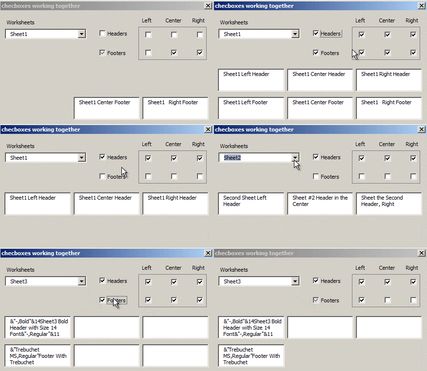
checkboxes working together

I’ve been working on a form with groups of checkboxes that perform pretty much the same action. All the checkboxes in a row are controlled by a “group” switch. Conversely, the group switch turns on or off, or goes to that grayed-out “Null” position, based on the state of its “member” checkboxes. Just like this worksheet header/footer preview form. In this case the group switches are the “Headers” and “Footers” checkboxes, with the member checkboxes to the right.

This form uses a collection of classes, one for each of the six member controls. Each class instance contains that single member control, along with a collection of all the member controls in the same row, and the row’s group checkbox. The class contains two event handlers: one for the member checkbox, and one for the group checkbox. To be able to create the event handlers, these two controls are declared using the WithEvents keyword.

The class looks like this:

'clsHeadFooterCheckboxes

Public WithEvents GroupCheckbox As MSForms.CheckBox
Public WithEvents MemberCheckbox As MSForms.CheckBox
Public collmemberCheckboxes As Collection
Public ParentForm As MSForms.UserForm

Private Sub MemberCheckbox_Click()
Dim ctl As MSForms.Control
Dim CheckedCheckboxCount As Long

'Avoid endless control click loops
If MemberCheckbox.Enabled Then
    'count the number of checked "member" controls
    For Each ctl In collMemberCheckboxes
        If ctl = True Then
            CheckedCheckboxCount = CheckedCheckboxCount + 1
        End If
    Next ctl

    With GroupCheckbox
        'Also avoid endless control click loops
        .Enabled = False
        'set the state of the group based on whether
        'all, no, or some members are checked
        .TripleState = False
        Select Case CheckedCheckboxCount
        Case 0
            .Value = False
        Case collmemberCheckboxes.Count
            .Value = True
        Case Else
            .TripleState = True
            .Value = Null
        End Select
        .Enabled = True
    End With
End If
SetTextBoxVisibility

End Sub

Private Sub GroupCheckbox_Click()
Dim ctl As MSForms.Control

'turn members on or off depending on group state
With GroupCheckbox
    'TripleState is only true when set by members
    'We don't want it to be available when clicking group
    .TripleState = False
    For Each ctl In collmemberCheckboxes
        'Avoid endless control click loops
        ctl.Enabled = False
        ctl.Value = .Value
        ctl.Enabled = True
    Next ctl
End With
SetTextBoxVisibility

End Sub

Sub SetTextBoxVisibility()
'Set the textboxes paired to the member controls visibility
ParentForm.Controls(Replace(memberCheckbox.Name, "chk", "txt")).Visible = memberCheckbox.Value
End Sub

While writing this code, I solved a problem that stumped me in the past: how to avoid looping of events when a pair of controls each triggers a change in the other. Application.EnableEvents doesn’t apply to userform controls, so you typically create some kind of EventsEnabled boolean variable. This is easy enough when only one control has a change event, but I’ve never been able to get it to work when two controls are affected by each other’s Change or Click events. This project was even more confusing, because events are triggered in three separate class instances, one for each member control in a row!

My solution was inspired by recent experience with VB.Net, where you can simply add and remove event handlers within your code. If you don’t want to trigger events, just unlink the control from its event handler, and add it back when you’re done. Obviously you can’t do that in VBA, but I realized I could disable a control before performing an action that would normally trigger its event. I did this in the MemberCheckbox_Click event. In the other direction it’s a little different. In the GroupCheckbox_Click event I disable the member checkbox and then check its state in the MemberCheckbox_Click event. This acts like an across-all-class-instances global variable that is tested in the groupCheckbox_Click event. I think. At any rate, it works.

Another tricky part was managing the group checkbox’s TripleState property. It only gets turned on in the MemberCheckbox_Click event, and only when some, but not all, of the member checkboxes are checked. This allows us to show a “grayed out” group checkbox. TripleState gets turned back off in the group checkbox’s click event, so when you are clicking it the only possibilities are checked or not checked.

This class is pretty flexible. You can add rows, or checkboxes within rows, and it works correctly. Just be sure to add the controls within the appropriate group and follow the naming pattern of the existing controls.

The userform code looks like this:

Private cHeadFooterCheckboxes As New clsHeadFooterCheckboxes
Private collCheckBoxClasses As Collection
Private WithEvents ThisBook As Excel.Workbook

Private Sub UserForm_Initialize()

Set ThisBook = ThisWorkbook
InitializeClasses
SetWorksheetCombo
SetDisplayTextBoxes
End Sub

Sub InitializeClasses()
Dim ctl As MSForms.Control
Dim RowName As String

Set collCheckBoxClasses = New Collection
'For each group control
For Each ctl In Me.grpgroupControls.Controls
    RowName = Replace(ctl.Name, "chkAll", "")
    InitializeRowClasses RowName
Next ctl
End Sub

Sub InitializeRowClasses(RowType As String)
Dim collRowmembers As Collection
Dim ctl As MSForms.Control

Set collRowmembers = New Collection
For Each ctl In Me.grpmemberControls.Controls
    'If it's a checkbox in the row being processed
    If InStr(ctl.Name, RowType) > 0 Then
        collRowmembers.Add ctl, ctl.Name
    End If
Next
'Create a class for each member control in the row
For Each ctl In collRowmembers
    Set cHeadFooterCheckboxes = New clsHeadFooterCheckboxes
    'initialize the class with the
    'control, other members and group
    With cHeadFooterCheckboxes
        Set .memberCheckbox = ctl
        Set .groupCheckbox = Me.Controls("chkAll" & RowType)
        Set .collmemberCheckboxes = collRowmembers
        Set .ParentForm = Me
    End With
    'add the class to the collection
    collCheckBoxClasses.Add cHeadFooterCheckboxes
Next ctl
End Sub

End Sub

Private Sub cboWorksheets_Change()
If Me.cboWorksheets.Enabled Then
    SetDisplayTextBoxes
End If
End Sub

Private Sub ThisBook_SheetActivate(ByVal Sh As Object)
SetWorksheetCombo
End Sub

There’s other code in the userform that handles the worksheet combobox. You can download a sample workbook to see it all in action.

Creating Dynamic Runtime Lists

I work in a world of lists. Lists that need to be reported on. Often these lists are implicit, in that they’re contained in the data that’s being processed and I don’t know in advance what, or how many, items they contain. In these situations, I determine the list by extracting it from the data right before processing it. That’s what I mean by creating dynamic runtime lists.

I first stumbled upon this concept when creating my FaceIdViewer. It was unique in that instead of hard-coding the number of FaceIDs in different versions of Excel, it just counted them up at runtime. Something like this code, which still works in Excel 2010.

Sub CountFaceids()
Dim cbar As Office.CommandBar
Dim ctl As Office.CommandBarControl
Dim FaceIdNumber As Long
Dim NoMoreFaceIds As Boolean

'the cbar probably doesn't exist, but if it does let's delete it
On Error Resume Next
Application.CommandBars("TempForFaceiIdCount").Delete
On Error GoTo 0
Set cbar = Application.CommandBars.Add(Name:="TempForFaceiIdCount", temporary:=True)
With cbar
    Set ctl = cbar.Controls.Add(Type:=msoControlButton)
    'FaceId index is zero-based
    FaceIdNumber = 0
    Do Until NoMoreFaceIds
        On Error Resume Next
        'Loop through the FaceId numbers, assigning them to the button,
        'until we error at the upper limit plus one
        ctl.FaceId = FaceIdNumber
        If Err.Number <> 0 Then
            NoMoreFaceIds = True
        End If
        On Error GoTo 0
        FaceIdNumber = FaceIdNumber + 1
    Loop
End With
Application.CommandBars("TempForFaceiIdCount").Delete
MsgBox Format(FaceIdNumber, "#,##0") & " FaceIds found"
End Sub


Excel 2010 FaceId count

(As an aside, it’s interesting that Excel 2010 has 22,716 FaceIds, more than double the 10,040 in Excel 2003, and thousands more than 2007, which has 16,210. I wonder why there’s such a big increase in something with such decreased use?)

Ice cream sales

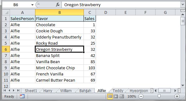
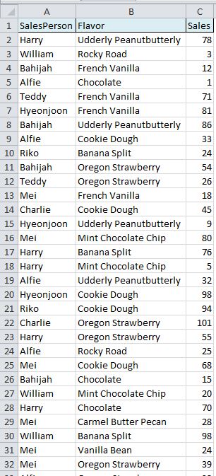
Another example of creating lists on the fly is splitting worksheets into multiple ones, based on the values in a certain column. It can be really hard to know beforehand what values will be in the column, as in this example of an ice cream store with multiple salespeople and, of course, many delicious flavors.

In addition to getting a list of salespeople in column A to report on, I want the list to contain unique entries. Each salesperson should only be listed once.

To get this unique list I use something like the function below. It stores the list in a collection, taking advantage of the fact that collections can’t contain duplicate keys. The function takes a range and adds each cell’s value to the collection, provided the value is unique. We surround the attempt with On Error statements, so that the code continues merrily along if trying to add a duplicate value causes an error. In this example it will quietly error many more times than not, generating a list of about 10 salespeople from the dozens of rows containing their names.

Function GetUniqueCellValues(rng As Excel.Range) As Collection
Dim collUniqueCellValues As Collection
Dim CellArray As Variant
Dim i As Long, j As Long

'assign all the cell values to a variant array
CellArray = rng.Value
Set collUniqueCellValues = New Collection
'cycle through the two dimensions of the array
For i = LBound(CellArray, 1) To UBound(CellArray, 1)
    For j = LBound(CellArray, 2) To UBound(CellArray, 2)
        'if we try to add a duplicate, ignore the error
        On Error Resume Next
        collUniqueCellValues.Add CStr(CellArray(i, j)), CStr(CellArray(i, j))
        On Error GoTo 0
    Next j
Next i
Set GetUniqueCellValues = collUniqueCellValues
End Function

The code above could just cycle through each cell in the range. Instead it loads the range’s values into a variant array and processes that array, which greatly speeds things up with long lists.

Below is an ice cream sales report subroutine that uses this GetUniqueCellValues function. It creates a collection containing each salesperson’s name. It then creates a new workbook to contain the individual reports. The source worksheet is copied to this workbook, once for each name in the collection. Each copied worksheet is filtered to show all names except the one being reported on. The visible rows are then deleted and the filter turned off. The result is a workbook with one report per salesperson. Note that, because we used a filter, no sorting is required:

Sub CreateSalesReports()
Dim wsSales As Excel.Worksheet
Dim wbSalesReport As Excel.Workbook
Dim ListLastRow As Long
Dim collSalesPeople As Collection
Dim i As Long
Dim wsSalesPerson As Excel.Worksheet

Set wbSalesReport = Workbooks.Add
Set wsSales = ThisWorkbook.Sheets("Sales")
With wsSales
    ListLastRow = .Range("A" & .Rows.Count).End(xlUp).Row
    'create the unique list/collection of salespeople
    Set collSalesPeople = GetUniqueCellValues(.Range("A2:A" & ListLastRow))
End With
'cycle through the salespeople, creating a worksheet/report for each
For i = 1 To collSalesPeople.Count
    wsSales.Copy after:=wbSalesReport.Sheets(wbSalesReport.Sheets.Count)
    Set wsSalesPerson = ActiveSheet
    'filter to all other salespeople
    With wsSalesPerson
        .Range("A1").AutoFilter Field:=1, Criteria1:="<>" & collSalesPeople(i)
        'delete the visible rows, leaving just those for the salesperson
        .Range("2:" & ListLastRow).EntireRow.Delete
        'name the worksheet
        .Name = collSalesPeople(i)
        .AutoFilterMode = False
    End With
Next i
End Sub


Here’s the resulting workbook:

If you’re interested, Dennis Wallentin explains a different way to get unique values from a range, using Advanced Filter.

Curbside Recycling

Free Dirt

Here in my beloved hometown there are many things available for free out on the sidewalks. Often they are marked by a sign.

More Free Stuff

And often they’re not, like this whimsical offering of fake flowers and sparkly stuff.

I’ve been getting in on the act lately and have deposited various furnishings on the curb out front. I always put signs on them, and because I’m silly I always come up with different way to say “Free.”

My favorite so far is “Free to a good home … or yours.” A more convoluted sign said “The state I’ve achieved tastes of reality.”

If I was to do it in Excel I guess I’d go with “=PMT(0,1,0)“.

Preview Excel Custom Formats


(Enter a format in column A and something in column B to preview the format.)

I was thinking of doing a simple post (hah!) on using Excel’s TEXT function to transform numbers to text, in order to match them to ID-type numbers from databases. One of my recurring work tasks is matching a host of possible school IDs from databases (text) to those in spreadsheets (numeric). I frequently use formulas like:

INDEX(tblFromCsv[School_Name],MATCH(TEXT(Numeric_ID,"0"),tblFromCsv[Text_Id],0))

Then recently a post here was featured on Chandoo’s site, along with some from other blogs – increasing my lifetime page views by about 30%. Searching his post for complimentary comments, I saw a couple along the lines of “Thanks for the great links, especially the one from Bacon Bits.”

Mike’s post is indeed a a beauty. It shows how to use custom number formats and create a percentage format like that shown in the first two rows of the interactive workbook above. It got me thinking about what formats you can specify in the TEXT function. It turns out anything you can enter as a custom format works for the TEXT’s Format argument, with very similar results. For example, this formula will format whatever’s in A1 with a format specified in B1:

=TEXT(A1,B1)

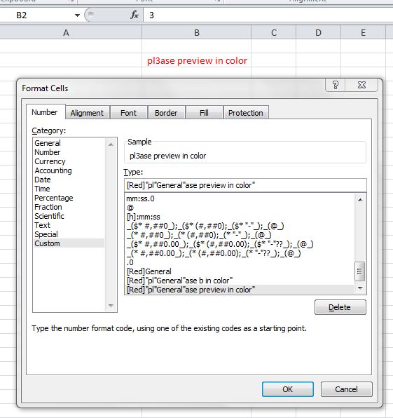
This got me thinking about creating a utility that shows the results of any custom format. Just like what you could get by using Excel’s custom format dialog or one line of VBA code, only a lot more work :). Although to be fair, Excel’s custom format dialog doesn’t show color:

Custom number format with no color preview

The reason TEXT doesn’t show color is that Excel functions – native and user-defined – don’t change the format of a cell. TEXT may seem like it’s breaking that rule, but it just returns a string that mimics the specified formatting.

So, adding color without VBA became my excuse reason for creating this tool. To do so, I used conditional formatting and an additional 29 columns of formulas. You can check them out by scrolling right in the workbook above. (You can also download it by using the button at the bottom of the workbook.)

There are two general types of custom formats, so my first task was to determine which kind is being used. The first has four different conditions in the form:

Positive number formats; negative number formats; zero formats; text formats

You can use less than four conditions. If you use only one, negative numbers and zero will use the positive format. If you use two, then zeros get the positive format.

The second type of custom form is more free-form and allows you to enter two custom conditions, and corresponding formats, along with a third format that covers all conditions not met by the first two. The conditions are specified using comparison operators enclosed in brackets like “[=]” “[<>]” “[>]”, etc. The form is:

1st condition and formats; 2nd condition and formats; formats for unmet conditions

Rows 4 through 6 above have some examples. Keep in mind that these custom conditions are evaluated from left to right, and when one is met the evaluation stops, like a VBA If statement.

This Microsoft page has a good explanation of the conditional formats including both of these types.

Determining which of the two types is being is used pretty easy. If the format contains any comparison operators inside of brackets then “Has custom conditions” in column H is true. I used an array formula that searches the format for one of the operators listed in D15:D20:

{=IF($F2,SUM((ISERROR(SEARCH(main!$D$15:$D$20,main!A2))=FALSE)*1)>0,"")}

The rest of the 29 columns contain equally convoluted formulas that tease out the various conditions and whether they have associated colors. These are summarized in columns J:M and N:Q.

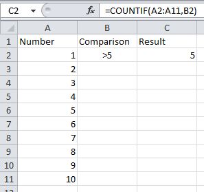
The conditional formatting uses COUNTIF. COUNTIF is the only function I know that understands comparison operators combined with numbers in a string. For example, if you have the numbers 1 to 10 in cells A1:A10 and “>5” in B1 you can do this:

Countif with comparison in cell

So I ended up with a conditional format for each possible color, like this:

=INDEX(N2:Q2,MATCH(1,COUNTIF(B2,J2:M2),0))="[Red]"

It’s an array formula, but for some reason in conditional formatting you don’t have to enter them with Shft-Ctrl-Enter and you don’t get the curly brackets. If anybody knows how conditional formatting recognizes array formulas, I’d like to hear.

I know of two things that don’t work correctly in this tool:

  • Text is sometimes colored when it shouldn’t be. If a text color isn’t explicitly implied it should not be changed, unless the general format is used for the positive condition. With this tool it uses the positive condition format in all cases.
  • If you put a color or custom condition, things that are enclosed in brackets, inside of quotes, this will still recognize them as colors or conditions. So don’t do that, at least for testing.

I could fix the first, but I’m not sure about the second. If you see any other failings, feel free to leave a comment.

I mentioned that this all could be done with one line of code. Assuming you have a number in A1 and format in B1, this line of code will apply the format to the number. Note that you need to format B1 as text so you can enter formats like 0000 – without quotes – and not have Excel convert them to a single zero.

Range("A1").NumberFormat = Range("B1")

I learned a ton from doing this, and now have a much more detailed understanding of custom formats. Have you done any projects that were less-than-practical, but rewarding?

Userform Application-Level Events

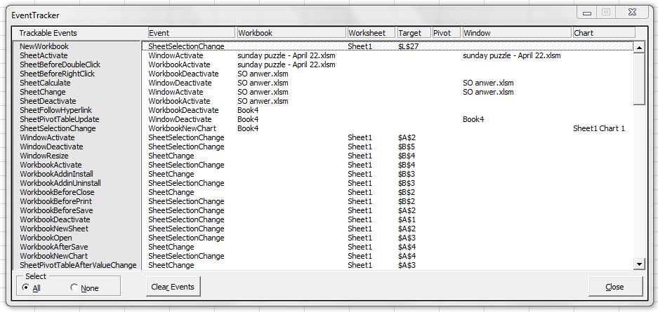
I’ve been fooling around with workbook and application-level events in UserForms. I’ve put them to good use in one or two projects, so thought I’d post about it. While thinking about the best way to present it, I ended up with a form that allows you to track all application-level events in an Excel instance. EventTracker looks like this (click the pic to for bigger one):

EventTracker in Action

Warning: meandering post ahead

curves ahead

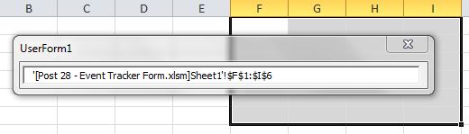
Before we get to that though, here’s how you can create a simple form that responds to all SheetSelectionChange events. First add a userform to a workbook in the Visual Basic Editor, then add a textbox to it. Paste this code into the form’s code module:

Private WithEvents app As Excel.Application

Private Sub UserForm_Initialize()
Set app = Application
End Sub

Private Sub app_SheetSelectionChange(ByVal Sh As Object, ByVal Target As Range)
Me.TextBox1 = Target.Address(external:=True)
End Sub

The code creates a WithEvents Application variable which is used to track application-level events. In this case, we’ll track the SheetSelectionChange event, but you can select other ones by selecting “app” in the dropdown at the top left of the VBA editor and the event in the dropdown at the top right.

Before you run the form you need to set its ShowModal property to False (or there will be no application-level events to track). Or you could just add this code to the code above:

Private Sub UserForm_Activate()
Static Activating As Boolean
If Activating = False Then
    Activating = True
    Me.Hide
    Me.Show vbModeless
End If
End Sub

I didn’t know the above would work until I tried it here. I don’t recommend it for any kind of serious coding, because of the static variable, but I like it. Basically the code only runs the first time UserForm_Activate runs. It hides the form and then shows it again modally, obviating the need to set the ShowModal property in design time or open the form from another module.

Now run the form and you’ll see that every SelectionChange event is reflected in Textbox1.

Simple event tracker form

So, back to the EventTracker form. It has two listboxes, one that shows all the available events to track, and one that lists the events that have occurred. You can set the events to track to all or none, or just some. The listbox is set to MultiSelectExtended, which means you can use Shift and Control to select ranges. I also added code so that Ctrl-A selects the whole list. Plus there’s option buttons!

The listbox that tracks events gets resized as they are added. (The form is resizable as well.) It shows the event and its parameters, such as the name of the worksheet being activated. I changed the parameters slightly, separating out the “Target” argument for the SheetPivotTableUpdate event into a “Pivot” column. The code that adds a row to the recent events uses a paramarray, which is the first time I’ve ever used one.

Here are some of the things I learned while making, and running, the form:

1. Even when the “After pressing enter, move selection” option is off, the SheetSelectionChange event fires after you edit a cell and hit Enter. Who knew?

2. There are a bunch of new events in Excel 2010. I only included “WorkbookAfterSave,” “WorkbookNewChart” and “SheetPivotTableAfterValueChange” in this tool. The rest have to do with Pivot table OLAP cubes.

3. There’s still no BeforeReallyClosing event though.

4. The maximum number of items allowed in a listbox is subject to available resources. On my laptop that equated to 6,242,685, so I didn’t need code to handle overfilling the event tracking listbox.

5. I discovered Chip Pearson’s excellent form resizing API code and used it to set the form with a minimize button and the ability to be resized.

One bit of code that’s useful on its own resizes column widths in a listbox. It’s based on this Daily Dose of Excel post, which in turn was based on a very thorough post by Jan Karel Pieterse. I modified Dick’s code to include the headers in the resizing, and also to base the the resizing only on the listbox’s visible rows:

Private Sub SetLstRecentEventsColumnWidths()

'Uses a hidden label in the form to hold
'text from headers and visible rows and
'resize to the widest one for each column

Dim ColWidths As String
Dim MaxWidth As Double
Dim i As Long
Dim j As Long
Dim VisibleRowsCount As Long
Dim HeaderLabels As Collection
Dim HeaderLabelWidths As Double

'create the HeaderLabels collection
Set HeaderLabels = GetHeaderLabels
With Me.lstRecentEvents
    'skip the code if no rows yet
    If .TopIndex > -1 Then
        VisibleRowsCount = Application.WorksheetFunction.Min((.ListCount - .TopIndex) - 1, .Height / lblHidden.Height)
        For i = 0 To .ColumnCount - 1
            'first get the header label width
            Me.lblHidden.Caption = HeaderLabels(i + 1) & "MM"
            MaxWidth = Application.WorksheetFunction.Max(Me.lblHidden.Width, MaxWidth)
            'only want to resize for the visible rows
            For j = .TopIndex To .TopIndex + VisibleRowsCount
                Me.lblHidden.Caption = .Column(i, j) & "MM"
                MaxWidth = Application.WorksheetFunction.Max(Me.lblHidden.Width, MaxWidth)
            Next j
            ColWidths = ColWidths & CLng(MaxWidth + 1) & ";"
            HeaderLabels(i + 1).Left = HeaderLabels(1).Left + HeaderLabelWidths
            HeaderLabels(i + 1).Width = MaxWidth
            HeaderLabelWidths = HeaderLabelWidths + CLng(MaxWidth + 1)
            MaxWidth = 0
        Next i
        .ColumnWidths = ColWidths
    End If
End With
End Sub

everywhere you go ...
Back to the EventTracker form again. As my father might say “The road is the destination.” Or is it “kindling is fire…?”

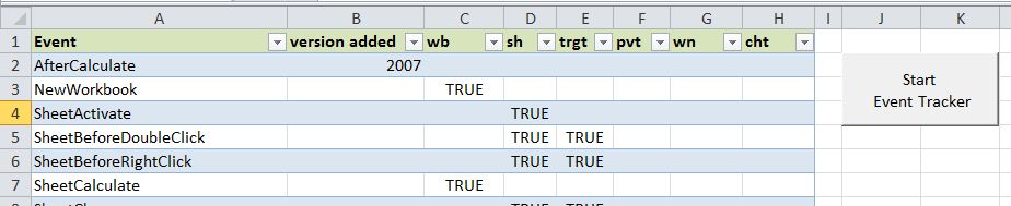
The downloadable zip file has a grid showing the events handled and a handy button to start Event Tracker. The workbook is .xlsm format, because if it was saved in .xls then the more recent events wouldn’t be available. You can still run it in XL 2003 as long as you’ve installed the compatibility pack. When running in an earlier version than 2010, events not supported in that version show up in the form module under “General,” rather than under “app.”

Event tracker workbook

User-Friendly Survey Without VBA

A few times a year I email workbooks containing surveys to people at about 80 schools. The overall process goes something like: I get a list of a couple of thousand records, which is then split into multiple per-school survey workbooks, which are then emailed to the schools. School staff complete the surveys and email them back. They are then merged back into one file and analyzed. Until we figure out some kind of web-based SharePoint-type system, this all works pretty well. I’ve mostly automated the emailing – adjusting subject lines, recipient lists, attachments and body on a per-school basis – and the splitting and re-merging is all push-button, so it’s a pretty efficient process.

The workbook/surveys are designed to be as user-friendly as possible, both for the people completing them and for the those analyzing the results. I use a combination of data validation and conditional formatting to guide the recipients. Ideally this might also include some VBA for things the data validation can’t handle, but it’s not worth confusion and maintenance issues that would result. So instead the workbooks contain additional conditional formatting that warns people when their data entry has gone astray. It also uses a concept I think of as conditional named ranges to provide appropriate data validation choices.

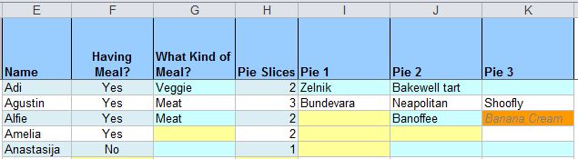
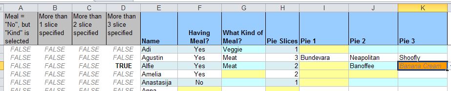
In the above picture, I’ve imagined some kind of International Pie Lovers Association, with a survey for their annual dinner. The meal choices are simple (Yes/No and Veggie/Meat) but they can choose up to three slices of pie, with a separate data validation dropdown for each slice. Yellow cells indicate where choices need to be entered. Orange indicates an error: cells that were entered when a condition called for it, but where that condition is no longer true, for example, under pie slices “3” was entered originally and “Banana Cream” was chosen, but then the number of slices was reduced to “2.”

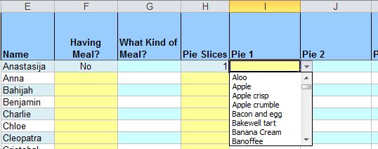
In order to make data entry more user-friendly, I came up with data validation which points at a named range that resolves to one or more cells if a condition is true, and to nothing if it’s not. In the picture below, the condition is true in the first cell in the “Pie 1” column and so a list of pies is available, but if you clicked the dropdown in the “Pie 2” column there would be no choices. That’s because the user chose 1 in the “Pie Slices” column, so the conditional range equates to nothing for the “Pie 2” column.

There are many ways to do condtional data validation and Debra Dalgleish has lots of great info on her website. In the dark days before I had my own blog she was kind enough to post about this particular conditional range concept.

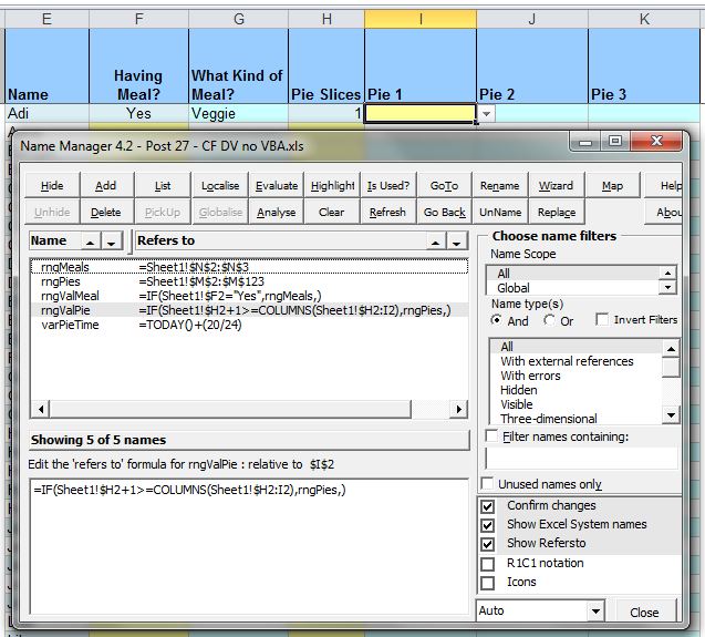
To set up the conditional range, I first create a named range called “rngPies” that points at a static list of pies in column M. Then I create the conditional range, called “rngValPie,” which points at rngPies if the condition is met, and points at nothing if it’s not. The formula for rngValPie (with I2 selected) is:

=IF(Sheet1!$H2+1>=COLUMNS(Sheet1!$H2:I2),rngPies,)

In English it says “If the number of slices selected is less than or equal to the number in this column, use rngPies, otherwise use nothing.” Here it is in the indispensable Name Manager.

The data validation then points at rngValPie. If a pie should be chosen the data validation shows the list, otherwise there’s no choices available.

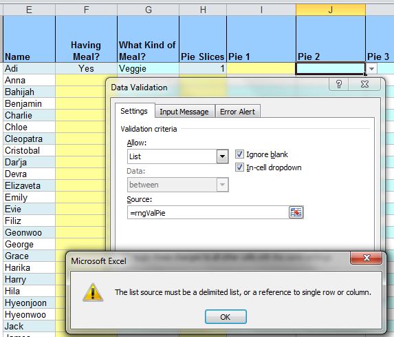
Note that when you enter a conditional range in the Data Validation dialog, the condition needs to be true, otherwise you’ll get an error message. For instance, if I try to enter the data validation while J2 is the active cell, I’ll see this:

Turning the cells orange if unneeded data is entered is accomplished with conditional formatting and some helper columns to the left of the data entry area.

The helper columns contain formulas that feed the conditional formatting. I could put the formulas from the helper columns directly in the conditional formatting, but do it this way because it’s easier for us back at the office to spot invalid data by filtering the helper columns.

This system works well for us and for the folks at the schools (at least as far as I can tell). The amount of user-helpfulness is in good balance with the ease of maintenance. If you’d like to look at a sample workbook that’s Excel 2003-2010 compatible, here’s the zipped file.

Note: for another use of conditional ranges, which has worked very well for me, see this Jan Karel Pieterse post on Daily Dose of Excel.

Copy Numbers With Formatting to Strings

The other day a co-worker needed to convert the formatted numbers in cells to text strings in the same cells – text strings that still looked like the formatted cells. For example, a cell with the number 12.34 formatted as a dollar amount would be converted to the string “$12.34”. The same number formatted for percent with two decimal points would become the string “1234.00%”. Formatted as a date, it would become the string “1/12/1900 8:09:36 AM”. In other words, he wanted text strings that contain what your eyes see in the formatted cell.

So that this… becomes that.

It’s subtle, but you can see that the converted cells are now left-aligned and many of them have the green triangle indicating “number stored as text.” And the ISNUMBER formula in D2 has switched from TRUE to FALSE.

My co-workder needed this because his worksheet was feeding an ArcGIS web-based map, with the cell values being used for interactive tables, or something like that. With formatted numbers in the cells, the tables would show 12.34 for the above examples. By converting the numbers to strings, the data were correctly formatted.

I don’t know of any way to do this without VBA. In Excel we are able to format cells as text, but if you just apply the Text format to numbers you lose the formatting. If you format target cells as Text and then copy your formatted source cells over them, the target cells assume the source cells’ formatting. Pasting as Values loses the formatting. Converting to a csv loses the formatting. So, I think VBA is required for this.

The VBA Range object has a Text property, which returns the contents of the cell as they appear to the human eye, exactly what we want. Using this property I was able to write a few lines of code and convert my co-worker’s spreadsheet:

Dim cell as Excel.Range
For Each cell In Selection
   CellText = cell.Text
   '@ is the Text format
   cell.NumberFormat = "@"
   cell.Value2 = CellText
Next cell

Since the number of cells was very small, this ran quickly and did what he wanted. The cells were now pushed into the interworld with their formatting intact.

Looping through cells as above is quite slow. Running it on 20,000 rows with 40,000 cells takes about 20 seconds on my laptop. Ideally, you want to assign all the cells to a variant array, process the elements of the array, and then plunk the array back into the range of cells.

I’ve done this with the Range object’s Value2 property before and wrote some code to do the same with Text. However, my variant array kept returning Null after doing something like:

Dim varCells as Variant
varCells = Selection.Text

I found this Charles Williams post where he points out that, unlike Value or Value2, assigning the Text property of a range to a variant array returns Null, unless all the cells have the same value and format.

So I changed the code to loop through the cells one at a time and assign their Text property to a two-dimensional String array. Fortunately, we can still assign the whole array back to a range.

Charles’ post revealed another interesting gotcha: when looping through cells’ Text properties and assigning them to an array your code gets progressively slower, but only if the range has rows with different heights in it. In my testing I noticed that even if all the rows are set back to the same height this weirdness persists.

The solution is to, every so often, select the cell that’s being processed. In my case, I chose to do it every 1000 rows. This won’t work if ScreenUpdating is set to False. This creates an additional reason to not process the cells one at a time, as all those writes back to the spreadsheet would slow things down even more.

(That’s a funky bug isn’t it? Makes you use Select in your code and leave Screenupdating on. I swear, when I started, I thought this would be a 400 word post! Nothing is simple in Excel, at least nothing I write about.)

One other issue is that if your columns are too narrow for a number and a cell is displaying “####”, the resulting text string will be “####”. I included a line in the code below to autofit the columns, but I’m not sure it will fix every situation.

With this code 20,000 rows with 40,000 cells takes about four seconds. This is only slightly worse than the three seconds it takes if the row heights are all the same and the Select fix isn’t needed, and much better than the 20 seconds if the row heights are different and Charles’ Select fix isn’t used.

Sub NumberToStringWithFormat(rng As Excel.Range)
Dim Texts() As String
Dim i As Long, j As Long

'This might prevent "###" if column too narrow
rng.EntireColumn.AutoFit
'Can't use variables in Dim
ReDim Texts(1 To rng.Rows.Count, 1 To rng.Columns.Count)
For i = 1 To rng.Rows.Count
    'Charles' fix for slow code with Text
    If i Mod 1000 = 0 Then
        rng.Range("A1").Offset(i).Select
    End If
    For j = 1 To rng.Columns.Count
        Texts(i, j) = rng.Cells(i, j).Text
    Next j
Next i
'@ is the Text format
rng.NumberFormat = "@"
rng.Value2 = Texts
End Sub

Regex Function to Sum Numbers in String

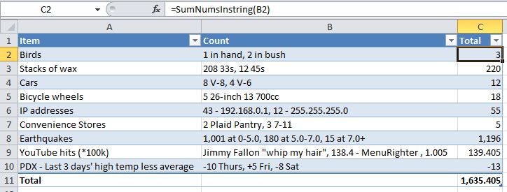
I recently needed to sum the numeric parts of strings in cells. For example, a cell with “4 calling birds, 3 dog night” would equal seven. So I came up with a regex function to sum numbers in strings. Actually, the regex identified the numbers, and the rest was easy.

The original version worked for things like the following: positive integers with no commas:

easy regex with just positive integers

For those of you not familiar with the basics of regex matching, here’s a short sample that takes a string like those above, applies a simple regex pattern for positive integers and sums the matches. It uses early binding, so you need to set a reference to “Microsoft VBScript Regular Expressions 5.5” in the VBE.

Sub BasicRegexFind()
'Set a reference to "Microsoft VBScript Regular Expressions 5.5"
Dim regex As VBScript_RegExp_55.RegExp
Dim rgxMatch As VBScript_RegExp_55.Match
Dim rgxMatches As VBScript_RegExp_55.MatchCollection
Dim StringToSearch As String

StringToSearch = "4 calling birds, 76 Trombones"

Set regex = New VBScript_RegExp_55.RegExp
With regex
    'Find all matches, not just the first
    .Global = True
    'search for any integer matches
    '"\d+" is the same as "[0-9]+"
    .Pattern = "\d+"
    'built-in test for matches!
    If .Test(StringToSearch) Then
        'if matches, create a collection of them
        Set rgxMatches = .Execute(StringToSearch)
        For Each rgxMatch In rgxMatches
          Debug.Print rgxMatch
        Next rgxMatch
    End If
End With

End Sub

The VBScript regex object is easy to work with, complete with a “Test” method that tells you if there’s any matches, and a collection of matches you can loop through with For/Next.

While the object is pretty straightforward, the concepts are confusing, and the syntax is nuts! I don’t know how much I’ll ever memorize. So before moving on to my voyage of discovery in developing a better function, here’s a couple of resources that helped me. The first site I turn to is regular-expressions.info. This link deals specifically with VBScript regex engine, but there’s many pages of tutorials on syntax and concepts. This tutorial by Patrick Matthews on Experts Exchange focuses on VBA and also contains a bunch of powerful regex-based “wrapper” functions you can use to match and replace text, without having to know how they work. Finally, you can take a look at the many masterful VBA/regex solutions provided by brettdj to real-world questions asked on stackoverflow.

The match pattern used above – “\d+” – worked for my original task, as I was adding only positive integers in strings with no other numbers of any sort. But what about…

  • sub-strings with numbers that shouldn’t be counted, like “Catch-22” or “7-Eleven”
  • decimal number
  • negative numbers
  • numbers with commas
  • non-numeric strings with nothing but numerals and periods, like IP addresses

In other words, we’re looking for substrings containing only numerals, periods, commas, or plus or minus signs. Further, after the optional plus or minus sign, any legitimate match must start with either a single digit or a decimal point followed by a digit.

Regular expressions includes a zero-length match construct – “\b” – that matches a “word” boundary. I thought something like “\b\d+\b” would match a positive integer bounded by a space. But it turns out that a period is a “non-word” character, so “192” and all the other numeric sections of “192.168.0.1” are seen as words and matched. Also, it would split decimal numbers into their integer and decimal parts, so 3.14159 would yield two matches of 3 and 14159, without the decimal. Alas, “\b” was no use to me. In addition, I realized that I was going to have to capture entire strings, such as IP addresses, because otherwise I’d generate a bunch of false positives from their parts. They’d need to be deleted from the real positives with an IsNumeric test after the regex matching was done.

Then I figured I could just check for a space preceding and following the match. That almost works, but since the space is part of the match, it only works for the first occurrence. With a string like “22 33” the space between 22 and 33 only gets counted as the space after 22. The regex doesn’t recognize that 33 has a space in front of it because it’s already moved on down the road.

What ended up working was a “Lookahead.” This is another zero-length match construct that checks the character following the pattern to be matched, without including it in the match. It sees the space at the end of 22, and it’s still available to be matched as the space at the beginning of 33. This is key, since the VbScript regex engine, unlike others, has no Lookbehind construct. So the pattern includes a Lookahead for a space. The positive Lookahead pattern for a space is (?= ).

Lookaheads also help ensure that commas only appear in reasonable places. One states that commas match only if they’re followed by three digits, the second only allows decimal points that aren’t followed by a comma. The negative Lookahead pattern for a comma is (!=,). (All of my comma and period usage here is US-centric and would need to be adjusted for those using different decimal marks or thousands separators).

Finally, the pattern only matches if it starts with a space or the zero-length begin-of-string construct, “^”. And, if the positive Lookahead for a space failed, it must end at the end-of-string ($). Here’s the full pattern:

(^| )[-+]?(\d|\.\d)(\d+|\.(?![.,])|(,(?=\d{3})))*((?= )|$)"

Broken down it says:

(^| )

– must begin with a space or be at the beginning of the string

[-+]?

– followed by zero or one occurrences of either a plus or minus sign

(\d|\.\d)

– followed by a single digit, or
a decimal point that’s followed by a single digit

(\d+|\.(?![.,])|(,(?=\d{3})))*

– followed by zero or more instances of
one or more integers, or
a decimal point that’s not followed by a decimal point or comma, or
a comma that’s followed by three integers

((?= )|$)

– match only if all of the above is followed by a space,
or if it’s at the end of the string

Since a valid match can have a space at the beginning the code includes a trim statement. It also strips out commas, which are allowed in the regex, but won’t pass IsNumeric. Here’s the complete function. It’s late-bound:

Function SumNumsInString(StringToSearch As String) As Double
'Finds numbers within a string and sums them
'Late-binding, so no reference needed

Dim regex As Object
Dim rgxMatch As Object
Dim rgxMatches As Object
Dim NumSum As Double

Set regex = CreateObject("vbScript.RegExp")
With regex
    .Global = True
.Pattern = "(^| )[-+]?(\d|\.\d)(\d+|\.(?![.,])|(,(?=\d{3})))*((?= )|$)"
'non-submatch-capuring version
'"(?:^| )[-+]?(?:\d|\.\d)(?:\d+|\.(?![.,])|(?:,(?=\d{3})))*(?:(?= )|$)"
If .Test(StringToSearch) Then
        Set rgxMatches = .Execute(StringToSearch)
        For Each rgxMatch In rgxMatches
            If IsNumeric(Replace(rgxMatch, ",", "")) Then
                NumSum = NumSum + Replace(rgxMatch, ",", "")
            End If
        Next rgxMatch
    End If
End With
SumNumsInString = NumSum
End Function

There’s also a Regexp.Submatch property – a collection that contains every submatch in the match, where a submatch is a piece of the pattern inside parentheses. So I could have checked if the first submatch was a space and only used the succeeding submatches. This would have eliminated the need to Trim the string, but seems more complex.

Since I didn’t use the submatches I could have included regex characters that tell the engine not the store them, speeding up the regex. Then the pattern would look like the commented one in the code, where the “?:” after each opening paren performs that function:

(?:^| )[-+]?(?:\d|\.\d)(?:\d+|\.(?![.,])|(?:,(?=\d{3})))*(?:(?= )|$)

That means there’s three types of question marks in one pattern: the ones just mentioned, the ones that follow “[-+}” and means to match it zero or one times, and the one that’s part of the Lookahead “?=” pattern. Whew!

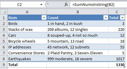
Anyways, here’s a more complex version of the first table, with the intended numbers being found:

Clearly this isn’t a foolproof function (D’oh!). My intent was firstly to learn about regexes while having fun, and also to outline my trial-and-error process in a way that may help others. So, although I researched concepts and syntax on the web, I didn’t look at anybody’s actual solutions for this type of function, as I wanted to just hack away on my own.

As always, I’m sure there’s a better way, and I’d love to hear yours!

Index/Sumproduct or Index/Match for Multiple Criteria Lookups?

You can use an INDEX/MATCH formula to look up an item in a list, as explained in this Contextures page. It’s trickier than a VLOOKUP formula, but it can look to the left and adjusts well when data columns are added or deleted. The generic layout of a single-criterion INDEX/MATCH is:

=INDEX(ColumnToIndex,MATCH(ItemToMatch, ColumnWithMatch, 0))

The MATCH section results in a row number that gets applied to the ColumnToIndex.

When looking up items with more than one criteria, I like to use an INDEX/SUMPRODUCT formula, replacing the MATCH part of the single criterion formula with SUMPRODUCT array multiplication, as descibed by Chandoo. Very generically that looks like:

=INDEX(ColumnToIndex,SUMPRODUCT(Multiply a bunch of columns and criteria))

This post started as an explanation of that approach. But in looking at the Contextures “INDEX/MATCH – Example 4” in the link above, I think it might be better. So this post is now a comparison of the two approaches.

Below is a live, downloadable worksheet with pairs of double-criteria lookup formulas – an INDEX/SUMPRODUCT and INDEX/MATCH in each case. Each row has two lookups: the first returns the number of home runs for that team and year, the second looks up a relative ranking.

I actually broke the formulas into two columns, which is what I’d do in a real project. Columns I and J contain INDEX formulas which refer to the lookup formulas in column H. The INDEX formulas first check if the lookup in column H actually returned a row. IF not “NA” is returned.

I break the lookup formula into two parts like this for a couple of reasons. The first is that if there’s no match the SUMPRODUCT in column H returns 0, which is important to see. The second is there’s often more than one formula referring to the calculated row, so it’s more efficient to only calculate it once and then use it in the different INDEX formulas. In this case the row is used for both the column I and column J INDEX formulas.

Here are the two lookup formulas, in cells H2 and H3, that are used to match the correct row. They are matching 2006 for the year and CHC for the team:

=SUMPRODUCT(($A$1:$A$33=$F2)*($B$1:$B$33=$G2)*(ROW($A$1:$A$33)-(ROW($A$1)-1)))
=MATCH(1,($A$1:$A$33=$F3)*($B$1:$B$33=$G3),0)

At their core they contain the same logic: ($A$1:$A$33=$F2)*($B$1:$B$33=$G2), which multiplies TRUEs and FALSES to return an array of Ones and Zeros. Here’s the SUMPRODUCT version with the above section evaluated by highlighting it and pressing F9. Note the 1 in the 19th position:

The SUMPRODUCT then multiplies that array times an adjusted row number, while the MATCH version finds the position of the number 1 in the array. Both result in row 19.

As mentioned above, the SUMPRODUCT formula returns 0 if no match is found. The INDEX formulas in columns I and J need to deal with that, otherwise they will return incorrect results. For example, if you have something like =INDEX({1,2,3,4,5},0), the result is 1. You might be surprised that it returns anything at all, but the nature of an INDEX formula is that if the row argument is set to 0 it evaluates the entire column. The actual row returned depends on the row of the formula. Confused? Me too.

The MATCH version, on the other hand, returns “#N/A” if no match is found, which is probably what you’d expect, and therefore good. And it’s shorter, also good. The only pitfall is that it’s an array formula and must be entered using Ctrl-Shft-Enter.

I’ve tried to make both sets of formulas more robust by including the headers in the ranges – $A1, $B1, etc. That way if a line in inserted below the header and before the first row of data, the formulas still work. I also want to ensure that the formulas still work if rows are inserted above the table’s header. This causes more complications in the SUMPRODUCT version, in the (ROW($A$1:$A$33)-(ROW($A$1)-1)) part. If you know the table will always start in Row 1 then it can be simplified to ROW($A$1:$A$33)-1. The MATCH version doesn’t have this issue.

Below the first pair of formulas are two more pairs, showing the results if no match is found, and if multiple matches are found. When there’s no match, the INDEX formula result in “NA” in both cases.

If there’s more than one match the SUMPRODUCT version adds together the matched rows. This results in 41 in row 12. Since 41 is outside the ColumnToIndex range, the result is #REF!. The MATCH version returns the first match. Obviously some kind of check for duplicates is good, such as the conditional formatting used here to highlight rows 20 and 21 of the data.

This being Excel, there are other ways to skin this cat. Here’s a post by JP Pinto, with his explanation of these two approaches, plus a LOOKUP version. (There’s a small error in the SUMPRODUCT version which is addressed in the comments.)

So which do I prefer now? Well, even though the MATCH version is simpler in most respects, I tend to avoid array formulas when possible, mainly because I too often forget that they are array formulas, do some editing, don’t hit Ctrl-Shft-Enter and have a moment, or several, of disorientation staring at the #N/A result. So I’ll probably stick with INDEX/SUMPRODUCT.

What do you think?

Solving the NPR Sunday Puzzle – #4

Not to brag but… well, okay, to brag, I had a personal best time in solving this week’s puzzle:

“Name two different kinds of wool. Take the first five letters of one, followed by the last three letters of the other. The result will spell the first and last name of a famous actor. Who is it?”

I could contrive a way to solve this with Excel, but I’m really just looking for an excuse to tell a riddle made up years ago, which provides a clue to the answer:

Q. What do you call a piece of luggage made from wool?

Continue reading →