Single Quotes in Worksheet Names

I was working on a function that uses regular expressions to determine whether a potential name for a workbook, worksheet or range contains illegal characters. I started by writing a little routine to determine which characters are illegal for sheet names. Of course, I could have just used one that I knew was prohibited and got the message below. But then I might never have thought about the use of single quotes in worksheet names.

Illegal worksheet character message

Here’s the code I used:

Sub IllegalWsNameCharacters()
Dim i As Long

With ActiveSheet
    .Range("A1").Cells.ClearContents
    For i = 0 To 127
        On Error Resume Next
        .Name = Chr(i)
        If Err.Number <> 0 Then
            .Range("A1").Value = .Range("A1").Value & Chr(i)
        End If
        On Error GoTo 0
    Next i
End With
End Sub

It cycles through each of the 128 ASCII characters and tries to use it as the ActiveSheet’s name. An error means that character is illegal, at least by itself, so it’s added to the contents of cell A1. I don’t know why I printed to a cell instead of the Immediate window, but it kept me from immediately (ha!) noticing that the first illegal character was a single quote or, as normal people say, an apostrophe.

Single quote in cell

You can see it doesn’t show up in the cell contents, only in the formula box. That’s because the single quote is the escape character that tells Excel that whatever follows it is text, and part of its duty is to stay quietly out of sight.

At any rate, I saw it and was surprised at it’s illegality. I’m pretty sure I’ve used an apostrophe in a sheet name before. And, sure enough you can:

Name with single quote

What you can’t do is use it as the first or last character in a sheet name. And this makes sense, since single quotes are how Excel surrounds worksheet and workbook names that have spaces in them, as in:

='A spaced out name'!A1 * serious_wks_name!A1

All in all, it seems you are best off leaving single quotes out of your sheet names. A quick web search reveals issues with hyperlinks, OLEDB references and Excel Services REST, whatever that is.

Finally, and interestingly, you can name your sheets with some of the “nonprintable” ASCII character codes, i.e., characters 0 to 31, if only through VBA:

ActiveSheet.Name = Chr(8) & " " & Chr(12) & " " & Chr(17) & " " & Chr(15) & " " & Chr(14)

Mind you, I’m not recommending it.

Worksheet name with nonprintable characters

Why Pi is Irrational – In Pictures

I was a good math student in junior high, and I’m sure I did well on all my pi-related homework and test questions. I understood that pi was an irrational number, and knew, theoretically, that it had an endless number of non-repeating decimals. However, I had no real grasp of why it’s irrational. It was just another abstract, memorized math fact. But a few years back a realization came to me. So, in belated celebration of Pi Day on March 14, I offer my pictorial explanation of why pi is irrational.

The realization came when thinking about the formula for an area of a circle, Π r2 (pi * r2) where r is the circle’s radius. It dawned on me that the r2 referred to a real geometric square with sides and corners and all, not just a letter with a number above it, and that:

Pi represents the number of squares with a side of length r that would fill a circle with a radius of length r.

Therefore, my explanation of why pi’s digits are infinite is that no matter how many squares you put inside a circle, there will always be a smaller “corner” into which you can cram a smaller square. This leaves an even smaller corner for an even smaller square, and on and on without end.

Pi Squares 1

I don’t know whether this is a mathematically valid explanation. But transforming this abstract concept into something I could draw with a pencil pleased me no end.

Pi and VBA

A pencil is one thing, but on Pi Day I decided to illustrate my explanation with Excel and VBA. It took me a really long time! First I tried using shapes, a reasonable, but really bad, idea. I ended up using just one shape, a circle, and a bunch of tiny cells, which are, after all, squares:

Pi Squares 2

The circle above has a radius of 50. When all the squares that fit are filled in, their total area is about 3.08 times that of a square with a radius of 50. In other words, it’s fairly close to pi. If I change the settings to a radius of 100, the number climbs above 3.1, but still short of pi.

Programming this was challenging and fun. Because of the nature of the project I coded some things more loosely than normal. There’s a bunch of global variables, and even a “Select Case True” statement.

I did a lot of Unioning and Intersecting in the code. One thing I rediscovered is a major glitch with the Union statement, which gives you an incorrect cell count for the Union of two overlapping ranges:

Union wrong count

Two Miscellaneous Things

My search for a screen-capture-to-animated-GIF program continues. I had been using Cropper, but it was unable to keep up with the circle’s “exit stage left” in the animation above. As you can see, I’m now trying ScreenCast-o-Matic, which has a nice interface, and both desktop and web versions. For $15 I can upgrade and remove their logo from the video, but when I tried this morning their website refused to take my money.

Finally, on Pi Day’s website it claims to be celebrated all around the world. It must be a fairly abstract reference in countries that use the, more logical, DMY date system, e.g., 14/3/2013.

Download!

Here’s a workbook with the code.

No IFs in Conditional Formatting Formulas

From time to time I’ll answer a question on Stack Overflow about a Conditional Formatting formula that includes an IF statement. Something like this:

=IF(A2=”Something”,TRUE,FALSE)

I’ll politely let them know you don’t need IFs in conditional formatting formulas, and that their formula can be reduced to something like:

=A2=”Something”

I’m going to go out on a limb and say there’s never a need for an IF in a conditional formatting formula.

Why “No IFs?”

What I usually say quickly in my answers is that the IF is implied by the fact that it’s a conditional formula. In other words, when you write the formula you’re telling the conditional formatting:

“If this condition is true, then apply the format, otherwise don’t apply it”. You only need the condition, the rest is a given.

Further, there will never be a reason for a nested IF. Nested IFs only apply when there are more than two possible outcomes. And again, in CF there can only be two: formatting applied or formatting not applied. You might very well, of course, use ORs and ANDs, as those allow you to narrow down the condition:

=AND(A2=”Something”,A3=”Else”)

But it’s still only one condition with two possible outcomes.

something else

VBA FormatConditions – Per-Row ColorScales, DataBars and IconSets

At the end of Conditional Formatting Per-Row Color Scales I said I’d be back with code to selectively copy IconSets and DataBars on a per-row basis as well. It took some doing but it’s now presentable. I learned a lot about programming these types of FormatConditions and I’m going to use this utility to generalize what I learned.

First, here’s a sample of the code in action. Some silly guy has added Icons, Data Bars and Color Scales to the values in Row 1. Now he’s copying only the ColorScales from that first row to the rows below:
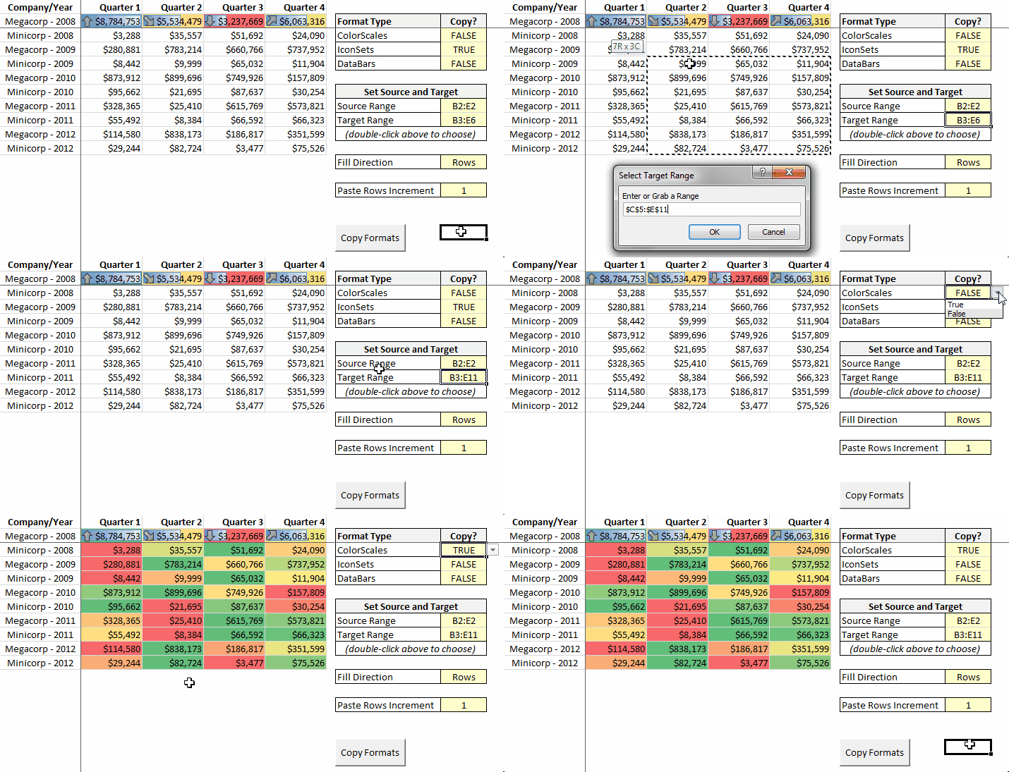
Conditional formatting copied

I (okay, it’s me) adjust the setting and push the button. The button routine passes the values in the worksheet to the main routine. It’s an expanded version of the code in the previous post, with an addition to delete selected formats. The main procedure is available in the download workbook linked at the end of this post. (The delete code is interesting, and shown later in this post.)

ColorScale, IconSet and DataBar Subroutines

Below are the three subroutines, called from the main procedure, to copy each type of FormatCondition: ColorScales, IconSets and DataBars.

The structure of each of these objects is different. With the exception of the Formula property, ColorScale has no relevant properties in the base object. The properties that need to be copied are all within its ColorScaleCriterion object. IconSets have relevant properties both within the IconSet object and within its IconCriterion object. Finally, DataBars contain no criterion object. All of its relevant properties are set within the base DataBar object.

ColorScale

Here’s the ColorScale subroutine. You can see that the only property in the ColorScale object is the Formula property, which is an interesting one. As far as I can tell this property is only applicable through code. I’ll discuss it more below. It’s only sometimes applicable, and if it’s not it will generate an error when you refer to it. So I surround it with and On Error statement to avoid that.

Sub SetRangeColorScale(rngTargetSection As Excel.Range, csSource As Excel.ColorScale)
Dim csTarget As ColorScale
Dim csCriterion As ColorScaleCriterion

Set csTarget = rngTargetSection.FormatConditions.AddColorScale(csSource.Type)
On Error Resume Next
csTarget.Formula = csSource.Formula
On Error GoTo 0
For Each csCriterion In csSource.ColorScaleCriteria
    With csTarget.ColorScaleCriteria(csCriterion.Index)
        On Error Resume Next
        .Type = csCriterion.Type
        On Error GoTo 0
        On Error Resume Next
        .Value = isCriterion.Value
        On Error GoTo 0
        .FormatColor.Color = csCriterion.FormatColor.Color
        .FormatColor.TintAndShade = csCriterion.FormatColor.TintAndShade
    End With
Next csCriterion
End Sub

Aside from Formula, the properties that need to be copied are part of ColorScale’s ColorScaleCriterion object. They are Type, and the Color and TintAndShade shade properties of ColorScaleCriterion.FormatColor.

The Type property specifies whether a criterion is based on a number, percent, percentile or formula. Value sets the value to be used for the Type, for example, the 90th percentile or the appropriate formula. These properties all have their counterpart in the conditional formatting dialog, shown here with a formula for the Min and Max values:

Color scale with formula

I surrounded the Type and Value assignments in an On Error statement because only some of the criteria have them and you’ll get an error on the ones that don’t. Sheesh, this stuff is confusing!

IconSet

Aside from Formula, the IconSet object has three properties that need to be copied: IconSet, ReverseOrder and ShowIconOnly. IconSet determines the color and type of icons and the others should be obvious:

Sub SetRangeIconset(rngTargetSection As Excel.Range, isSource As Excel.IconSetCondition)
Dim isTarget As IconSetCondition
Dim isCriterion As IconCriterion

Set isTarget = rngTargetSection.FormatConditions.AddIconSetCondition
With isTarget
    On Error Resume Next
    .Formula = isSource.Formula
    On Error GoTo 0
    .IconSet = isSource.IconSet
    .ReverseOrder = isSource.ReverseOrder
    .ShowIconOnly = isSource.ShowIconOnly
    For Each isCriterion In isSource.IconCriteria
        With .IconCriteria(isCriterion.Index)
            .Icon = isCriterion.Icon
            On Error Resume Next
            .Type = isCriterion.Type
            On Error GoTo 0
            On Error Resume Next
            .Value = isCriterion.Value
            On Error GoTo 0
            .Operator = isCriterion.Operator
        End With
    Next isCriterion
End With
End Sub

At the IconCriterion level, there are four properties: Icon, Type, Value and Operator. Icon allows you to change individual icons, just like you can in the user interface. For example, here the gray arrow icon set has been modified to use a green ball in place of the gray up arrow:

Changed icon

Operator sets the relationship of the Icon to the Value. For example, the “>” Operator says to use an up arrow if the cell’s value is greater than the Value property.

DataBar

The DataBar object has no criterion property. All the relevant properties are at the DataBar level. So instead of criteria for the Min and Max, you get the MinPoint and MaxPoint properties. These two made me nervous when I first saw them, as you have to set them via their Modify methods, but that seems to work fine.

Sub SetRangeDataBar(rngTargetSection As Excel.Range, dbSource As Databar)
Dim dbTarget As Databar

Set dbTarget = rngTargetSection.FormatConditions.AddDatabar
With dbTarget
    On Error Resume Next
    .Formula = dbSource.Formula
    On Error GoTo 0
    With .AxisColor
        .Color = dbSource.AxisColor.Color
        .TintAndShade = dbSource.AxisColor.TintAndShade
    End With
    .AxisPosition = dbSource.AxisPosition
    .BarBorder.Type = dbSource.BarBorder.Type
    With .BarColor
        .Color = dbSource.BarColor.Color
        .TintAndShade = dbSource.BarColor.TintAndShade
    End With
    .BarFillType = dbSource.BarFillType
    .Direction = dbSource.Direction
    .MinPoint.Modify newtype:=dbSource.MinPoint.Type, newvalue:=dbSource.MinPoint.Value
    .MaxPoint.Modify newtype:=dbSource.MaxPoint.Type, newvalue:=dbSource.MaxPoint.Value
    .NegativeBarFormat.ColorType = dbSource.NegativeBarFormat.ColorType
    With .NegativeBarFormat.Color
        .Color = dbSource.NegativeBarFormat.Color.Color
        .TintAndShade = dbSource.NegativeBarFormat.Color.TintAndShade
    End With
    .PercentMax = dbSource.PercentMax
    .PercentMin = dbSource.PercentMin
    .ShowValue = dbSource.ShowValue = True
End With
End Sub

There’s a whole bunch of properties besides MinPoint and MaxPoint. About half deal with formatting, including formatting of negative values. All of these are analogous to their similarly-named user interface properties:

Data bar dialog

Deleting Selected FormatConditions

I wrote a routine to delete only certain types of format conditions from a target range. It gets called before the routine to copy the formats. For example, if the routine is copying DataBar formats, we’ll first delete all the existing ones.

It took longer than I expected to get a workable routine, chiefly because my initial attempts were inpossibly slow. Whereas copying all three types of FormatCondition to 1000 rows takes about a second, deleting formats by looping through the whole FormatConditions collection was taking minutes.

The solution was to break the target range into little ranges of 10 rows each and delete the matching conditions from those ranges. I assume this must simplify Excel’s internal indexing of the FormatConditions collection, whatever that means :). This only takes a couple of seconds for a thousand rows.

The other thing to note is that you have to loop backwards through the FormatConditions – just like deleting any Excel object in a loop – or you’ll get a “Subscript out of Range” error:

Sub DeleteFormatConditions(rngTarget As Excel.Range, _
    DeleteColorScales As Boolean, DeleteDataBars As Boolean, DeleteIconSets As Boolean)
Dim FormatConditionsCount As Long
Dim DeleteIncrement As Long
Dim DeleteRangeStart As Long
Dim DeleteRangeEnd As Long
Dim DeleteDone As Boolean
Dim rngDelete As Excel.Range
Dim objFormatCondition As Object
Dim i As Long

'Break target range into smaller ranges, which makes deletion go many times faster!
DeleteIncrement = 10
DeleteRangeStart = 1
'Min to keep from going past end of target range
DeleteRangeEnd = Application.WorksheetFunction.Min _
    (DeleteRangeStart + DeleteIncrement, rngTarget.Rows.Count)
Do While Not DeleteDone
    'rngTarget.Parent is the worksheet
    Set rngDelete = rngTarget.Parent.Range(rngTarget.Cells(DeleteRangeStart, 1), _
        rngTarget.Cells(DeleteRangeEnd, rngTarget.Columns.Count))
    FormatConditionsCount = rngDelete.FormatConditions.Count
    'Check each format condition's type and call matching routine
    'Step backwards or risk "Subscript out of Range"
    For i = FormatConditionsCount To 1 Step -1
        Set objFormatCondition = rngDelete.FormatConditions(i)
        If DeleteColorScales And objFormatCondition.Type = 3 Then
            objFormatCondition.Delete
        End If
        If DeleteDataBars And objFormatCondition.Type = 4 Then
            objFormatCondition.Delete
        End If
        If DeleteIconSets And objFormatCondition.Type = 6 Then
            objFormatCondition.Delete
        End If
    Next i
    If DeleteRangeEnd >= rngTarget.Rows.Count Then
        DeleteDone = True
    End If
    DeleteRangeStart = Application.WorksheetFunction.Min _
        (DeleteRangeStart + DeleteIncrement, rngTarget.Rows.Count)
    DeleteRangeEnd = Application.WorksheetFunction.Min _
        (DeleteRangeEnd + DeleteIncrement, rngTarget.Rows.Count)
Loop
End Sub

The Formula Property

As I mentioned above, each of these FormatConditions has a Formula property. I don’t see a match for this property anywhere in the Excel user interface. According to MSDN, it:

Returns or sets a String representing a formula, which determines the values to which the data bar will be applied.

This property is useful to limit the range of values that will display the conditional format. A typical scenario is when you have a range of numbers containing both positive and negative values. You may want to create more than one conditional format for this range of numbers—one for positive values and another for negative values.

Sure enough, if I apply it to a DataBar definition, like so…

dbDataBar.Formula = "=A1 > -5"

… I get this formatting, where the DataBars are only applied to cells with values greater than negative 5:

Data bar formula property

If there is a way to do this in the user interface, please let me know!

Miscellaneous:

  • In my previous post on this, I noted that a recorded macro sets the added conditional format to the first priority and that I was doing the same in my code. However, that’s a bad idea. When copying more than one format it will rearrange their order.
  • If you are fooling around with this stuff, you’ll notice that recording a macro that modifies existing conditional formatting produces all the code for that formatting, not just for the modification. This can be annoying or useful, depending.
  • The StopIfTrue FormatConition doesn’t apply to these three objects. You can see that they are grayed out in the Excel dialog.
  • The ScopeType and PTCondition properties have to do with conditional formatting in pivot tables.

Download!

Here’s a workbook with a working model and all the code.

many borders fast

If you want to draw borders fast in Excel, you can hold down the Ctrl key, select all the areas that need borders and apply them in one swell foop!

many borders

I just realized this recently. It’s pretty fast, unless you’re trying to do a screen capture with buggy software.

Speaking of which, I just found a new straight-to-animated-gif program, called Cropper, that replaced the free-for-one-month-and-then-pay-$300 software (had it for a month.) Cropper works fine so far, except for one major bug. It’s not the most intuitive program, but on the flip side it works with no intermediate steps and produces a pretty small file.

Small enough, that is, that it loads pretty fast on my laptop. I’d be interested to hear from anybody about whether it started fast, or not, for them.

If you do use it, you’ll want to know about the bug. You can start a screenshot in at least two ways, double-clicking or pressing Alt-PrtSc. Double-clicking leaves the transparent blue selection layer on the screen, so I like the hotkey approach. But the bug is that the first time after opening Cropper, you need to start your capture by double-clicking or you’ll see the disheartening .Net runtime error screen.

Cropper error

After seeing it a few times the phrase “come a cropper” leapt to mind. But no worries, after double-clicking once you can use the hotkey for subsequent captures.

If anybody has any suggestions for animated gif software, I’m all ears.

Conditional Formatting Per-Row Color Scales

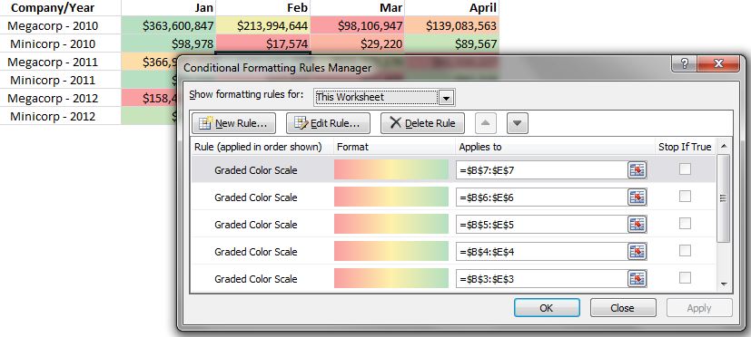
If you want to compare all the numbers in a range, you can apply a conditional formatting color scale to the entire area and it works just fine. However, sometimes I want to compare the data on a per-row basis. Here’s two examples of data that could use per-row color scales:

same color scale throughout 11

The first, above, mixes values and percents. All the percents are red – the low end of the scale – because they equate to numbers between 0 and 1, and they’re getting compared to sales values between 1 and 100.

same color scale throughout 2

The second mixes sales from a large and small business. The sales for the small business are all shown as low – red – because they’re generally less than 1/100th of the sales of the large corporation.

In both cases I just want to compare the cells in each row to each other. Doing that, the second example looks like this, showing the relative sales within the company and year:

per row color scale 1

VBA to Apply Per-Row Color Scales

As far as I can tell, there’s no quick built-in way to apply color-scales (or icon sets or data bars) on a per-row basis. Instead you need to apply them one row at a time. So, of course, I wrote some VBA.

I’ve long been intimidated by Excel 2010’s conditional formatting object model, at least when it comes to non-formula conditions. But one day I answered this StackOverflow post about per-row color scales and decided to dig deeper.

For that answer I turned on the Macro Recorder, applied a color scale, and then called the generated code in a loop for each row. A better approach is to copy an existing row with the color scale you want and paste it over each row.

The simplest version of this is to copy all formatting in a source row and paste it to a target row. However, I’d prefer to grab only the color scale and paste it, ignoring other formats such as borders, text styles and other conditional formats.

If you turn on the Macro Recorder and apply a 3-gradient color scale to a range, you get something that looks like this, with the last five lines repeated two more times:

Selection.FormatConditions.AddColorScale ColorScaleType:=3
Selection.FormatConditions(Selection.FormatConditions.Count).SetFirstPriority
Selection.FormatConditions(1).ColorScaleCriteria(1).Type = _
        xlConditionValueLowestValue
With Selection.FormatConditions(1).ColorScaleCriteria(1).FormatColor
    .Color = 7039480
    .TintAndShade = 0
End With

Note that it adds a ColorScale and then moves it to the top of the conditional formatting stack with SetFirstPriority.

I discovered a quirk when I tried to modify the above code to do some simple looping through the conditional formatting settings in a range. I tried something like this:

Dim fc As FormatCondition
For Each fc In Selection.FormatConditions
    Debug.Print fc.Application.Name
Next fc

That makes sense right? Set an object to a FormatCondition in order to loop through all the FormatConditions. However, if Selection only has color scale conditional formatting, you’ll get a “Type Mismatch” error on the “For Each fc” line. Turns out you need to declare fc as a ColorScale. Then the above code will run and will only cycle through the ColorScale objects.

So here’s the workhorse of my code. It’s called by the main module and loops through a target range, applying the color scale from the source range:

Sub SetRangeColorScale(rngTargetSection As Excel.Range, csSource As Excel.ColorScale)
Dim csTarget As ColorScale
Dim csCriterion As ColorScaleCriterion

Set csTarget = rngTargetSection.FormatConditions.AddColorScale(csSource.Type)
rngTargetSection.FormatConditions(rngTargetSection.FormatConditions.Count).SetFirstPriority
For Each csCriterion In csSource.ColorScaleCriteria
    With csTarget.ColorScaleCriteria(csCriterion.Index)
        .Type = csCriterion.Type
        .FormatColor.Color = csCriterion.FormatColor.Color
        .FormatColor.TintAndShade = csCriterion.FormatColor.TintAndShade
    End With
Next csCriterion
End Sub

Below is my main routine. It allows you to choose Row or Column orientation, so you can paste the color scales by-column if you wish. The SectionIncrement variable specifies how many rows at a time to paste the color scale, so you could apply the comparison over two or more rows (or columns) at a time.

Note that in this module, objSourceCondition is declared as an object and tested to see if it’s a ColorScale type of FormatCondition:

Sub CopyColorScaleInSections()
Dim rngSource As Excel.Range
Dim rngTarget As Excel.Range
Dim ws As Excel.Worksheet
Dim objSourceCondition As Object 'we'll test for ColorScale
Dim rngTargetSection As Excel.Range
Dim FillDirection As String
Dim IncompatibleRangeError As String
Dim SectionIncrement As Long
Dim SectionsCount As Long
Dim i As Long

'change the settings below to suit
Set ws = ActiveSheet
Set rngSource = ws.Range("B2:E2")
Set rngTarget = ws.Range("B3:E7")
FillDirection = "Rows"
SectionIncrement = 1

'deletes all existing formats
'you might want to change to just delete
'ColorScales, but for demo purposes
'this works well
rngTarget.FormatConditions.Delete
'checks whether the settings above work together
If Not CompatibleRanges(rngSource, rngTarget, SectionIncrement, _
        FillDirection, IncompatibleRangeError) Then
    MsgBox IncompatibleRangeError, vbOKOnly + vbExclamation
    GoTo exit_point
End If

'determine how many sections of rows or columns
'we'll be pasting over
If FillDirection = "Rows" Then
    SectionsCount = rngTarget.Rows.Count / SectionIncrement
ElseIf FillDirection = "Columns" Then
    SectionsCount = rngTarget.Columns.Count / SectionIncrement
End If

For i = 0 To SectionsCount - 1
    'set an individual section to be pasted over
    If FillDirection = "Rows" Then
        Set rngTargetSection = rngTarget((i * SectionIncrement) + 1, 1) _
            .Resize(SectionIncrement, rngTarget.Columns.Count)
    ElseIf FillDirection = "Columns" Then
        Set rngTargetSection = rngTarget(1, (i * SectionIncrement) + 1) _
            .Resize(rngTarget.Rows.Count, SectionIncrement)
    End If
    For Each objSourceCondition In rngSource.FormatConditions
        'test if it's a ColorScale - 3
        If objSourceCondition.Type = 3 Then
            SetRangeColorScale rngTargetSection, objSourceCondition
        End If
    Next objSourceCondition
Next i

exit_point:
End Sub

Obviously, when you do this you end up with a passel of conditional formatting rules, so don’t be surprised!

rule for each row

Here’s the function, called from the main routine above, that checks whether the source and target ranges are compatible:

Function CompatibleRanges(rngSource As Excel.Range, rngTarget As Excel.Range, _
    SectionIncrement As Long, FillDirection As String, _
    ByRef IncompatibleRangeError As String) As Boolean

'no #DIV/0
If SectionIncrement = 0 Then
    IncompatibleRangeError = _
    "You can't use an increment of 0"
    GoTo exit_point
End If
'can't specify a SectionIncrement bigger than the target range
If (FillDirection = "Rows" And rngTarget.Rows.Count < SectionIncrement) Or _
   (FillDirection = "Columns" And rngTarget.Columns.Count < SectionIncrement) Then
    IncompatibleRangeError = _
    "Target range must have at least" & vbCrLf & _
        SectionIncrement & " rows."
    GoTo exit_point
End If
'target range rows or columns must be
'evenly divisible by the SectionIncrement
If (FillDirection = "Rows" And rngTarget.Rows.Count Mod SectionIncrement <> 0) Or _
   (FillDirection = "Columns" And rngTarget.Columns.Count Mod SectionIncrement <> 0) Then
    IncompatibleRangeError = _
    "Target range " & FillDirection & " must be" & vbCrLf & _
         "evenly divisible by " & SectionIncrement & "."
    GoTo exit_point
End If
'target range width or height has to match
'source range width or height
If Not (rngSource.Rows.Count = rngTarget.Rows.Count Or _
        rngSource.Columns.Count = rngTarget.Columns.Count) Then
    IncompatibleRangeError = _
    "Source and Target ranges must have" & vbCrLf & _
        "either the same number" & vbCrLf & "of rows or columns."
    GoTo exit_point
End If

exit_point:
CompatibleRanges = IncompatibleRangeError = ""
End Function

I’ve run this code successfully on up to 10,000 rows. It took about 7 seconds. I did notice that deleting 9,900 of those rows afterwards takes a while, and that the workbook can then act sluggish until it’s saved. I’m not sure what the issue is.

No download right now, but I’m planning to whip up a workbook that expands this to IconSets and DataBars and whatever else I can cram in there. So look for that in a week or so.

Conditional Formatting Color Scales Based on Other Cells

With formula-based conditional formatting, it’s pretty easy to base the formats on other cells in the workbook, simply by referring to those cells in the formula. However, it’s more complicated if you want color scales derived from values in another range. In this post I discuss two ways to base color scales on another range. The first uses the camera tool while the second is a VBA subroutine that mimics conditional formatting.

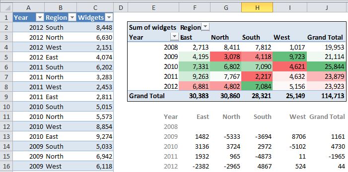
Below is an example of what I’m talking about. The color formatting isn’t based on the values in the pivot table. Instead, it reflects the values in the second table, each cell of which contains the difference from the previous year in the pivot table. The colors range from red at the low end to green at the high end:

ormat with camera tool 1

So, here’s my two approaches to doing this:

Using the Camera Tool

This method uses Excel’s under-publicized camera tool, which creates a live picture linked to a group of cells. In this case the formatting is applied to a pivot table, but you can do it with any range. Here’s the steps:

  • Create the range of formulas that you’ll base the conditional formatting on.
  • Format the numbers in that range to be invisible, by using a custom format of “;;;”. All you want to see is the conditional formatting.
  • Use the camera tool to take a picture of the entire pivot table and paste it over the range you just created, lining up the conditionally formatted cells. Set the picture to be completely transparent, using the “no fill” setting. This way you can see through the picture to the conditionally formatted cells underneath.

The result will be like the illustration below. The source pivot table is in rows 11 to 18, and you can see that the picture starting in row 2 is linked to it. The cells underneath the picture contain the formulas referring to the pivot table. The conditional formatting is based on these cells, whose text is invisible because of the custom format.

format with camera tool 2

One thing to be aware of is that the picture doesn’t update until there’s a worksheet recalculation. You may have to force recalculation with F9 to have the picture update.

For one project I augmented this method by writing code that let me toggle back and forth between the values in the pivot table and the values the conditional formatting is based on.

Using VBA to Create “FauxMatting”

As the heading implies, this method attempts to replicate conditional formatting using VBA. The following subroutine takes two ranges – a source and a target range – as its arguments. It finds the highest and lowest values in the source range. It assigns each of those values a color in a scale from green to red, with white in the middle. This is done by dividing the range of values source values into 255 increments. The colors are then assigned to the target range:

Sub ConditionalFauxmatting(rngSource As Excel.Range, rngTarget As Excel.Range)
Const NUMBER_OF_INCREMENTS As Long = 255
Dim MinValue As Double
Dim MaxValue As Double
Dim ScaleIncrement As Double
Dim ScalePosition As Long
Dim var As Variant
Dim CellColor() As Long
Dim i As Long, j As Long

If Not (rngSource.Rows.Count = rngTarget.Rows.Count And rngSource.Columns.Count = rngTarget.Columns.Count) Then
    MsgBox "Source and Target ranges must be" & vbCrLf & "same shape and size"
    GoTo exit_point
End If
MinValue = Application.WorksheetFunction.Min(rngSource.Value)
MaxValue = Application.WorksheetFunction.Max(rngSource.Value)
'divide the range between Min and Max values into 255 increments
ScaleIncrement = (MaxValue - MinValue) / NUMBER_OF_INCREMENTS
'if all source cells have the same value or there's only one
If ScaleIncrement = 0 Or rngSource.Cells.Count = 1 Then
    rngTarget.Cells.Interior.Color = RGB(255, 255, 255)
    GoTo exit_point
End If
'assign all the values to variant array
var = rngSource.Value
ReDim CellColor(UBound(var, 1), UBound(var, 2))
For i = LBound(var, 1) To UBound(var, 1)
    For j = LBound(var, 2) To UBound(var, 2)
        'the scale position must be a value between 0 and 255
        ScalePosition = (var(i, j) - MinValue) * (1 / ScaleIncrement)
        'this formula goes from blue to red, hitting white - RGB(255,255,255) at the midpoint
        CellColor(i, j) = RGB(Application.WorksheetFunction.Min(ScalePosition * 2, 255), _
        IIf(ScalePosition < 127, 255, Abs(ScalePosition - 255) * 2), _
        IIf(ScalePosition < 127, ScalePosition * 2, Abs(ScalePosition - 255) * 2))
    Next j
Next i
'assign the colors stored in the array
'to the target range
With rngTarget
    For i = 1 To .Rows.Count
        For j = 1 To .Columns.Count
            .Cells(i, j).Interior.Color = CellColor(i, j)
        Next j
    Next i
End With

exit_point:
End Sub

The result looks like this:

format with VBA

I’m not sure how practical this is, but it was fun to figure out! Obviously, you’d want to tie this to a worksheet or pivot table event to update the formatting when the values change.

Here’s a workbook demonstrating these two methods.

Unified Method of Pivot Table Formatting

In preparation for my big annual reporting push I’ve developed a (partial) Unified Method of Pivot Table Formatting. My motivation was to define a system that allows me to copy pivot tables as values while preserving the formatting, and that increases formatting flexibility. Simply stated the Unified Method is:

“Use Conditional Formatting for Everything, and Apply Every Conditional Format to the Entire Pivot Table.” *

That’s right. No built-in “PivotTable Styles,” no field-level conditional formats, and no more just selecting the whole table, drawing a border around it and hoping “Preserve cell formatting on update” works.

* Excel 2007 and later. Applies only to formula-based conditions, e.g., not to color scales. Other restrictions apply.

Formatted Pivot Table

Above is a section of a world population pivot table. It has the following conditional formats:

  • The header row is colored orange with a black border around each cell.
  • There’s a black border to the left and right of the table.
  • Subtotal rows are bold with a black border above and below but no interior border, and are the same color as the header row.
  • Detail row cells are surrounded by a light gray border.
  • There are no borders between columns A and B, as Column A is only one pixel wide and flops over into Column B, as with “Oceania Total.”
  • Country rows have alternate banding by country.
  • State/Province rows’ population number font is gray

That’s quite a list, I think you’ll agree. In the past I might have used regular formatting, pivot table styles and field-level conditional formatting. I’d like to avoid all of those approaches, for the following reasons:

Regular Formatting: By “regular formatting” I mean something like selecting the whole pivot table and applying an outside border. This requires the pivot table setting “Preserve cell formatting on update” to be turned on. I’ll admit I’ve never mastered the quirks of this setting, so I’d like to just avoid it.

I’ve already found things, like header row word-wrapping, that may make me relent on this one.

Built-in PivotTable Styles: I really don’t like the built-in pivot table styles, for a few reasons:

  • The text and cell colors are ugly to the point of unusability. They almost always need modification.
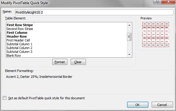
  • Modifying them is a pain. The names for pivot table parts are weird. For example, what’s a “First Row Stripe,” and how does “Column Subheading 2” compare to “Subtotal Column 2?” So I do a lot of guessing and backing out of the dialog to see if I guessed right. Very clunky.
  • Pivot Table Modify Style Dialog

  • Finally, if you copy the pivot as values these formats disappear, although John Walkenbach has a solution for that.

Field-level Conditional Formatting: The field-level conditional formatting that became available in Excel 2007, and that I discuss in Re-Apply Pivot Table Conditional Formatting, is certainly better than the pivot table styles. But, again, the formats disappear when you copy the pivot table as values. And you can only use them to format the value fields of a pivot table, so for something like alternate row banding that includes row labels you need to apply the rule twice.

THE “UNIFIED” APPROACH
So, instead of the approaches above, I apply every conditional format to the entire pivot table. I use the ModifyAppliesToRange method, as discussed in the post linked above, to re-apply conditional formatting to the entire pivot table when it’s refreshed. This keeps all the formatting intact when I copy the table as values. It also allows me to easily apply formatting to specific columns and rows.

Note that in the Extend Pivot Table Conditional Formatting Post I only dealt with the rows of the pivot table that had data. In the example file at the end of this post I’ve extended the code to include the entire pivot table.

Two Examples
Since I’m applying the conditional formatting to the whole pivot table, the conditions sometimes need to specify row or column numbers. For example, I only want to gray the text for State/Province rows in columns D and E. That condition looks like this:

=AND(COLUMN(A1)>=4,$C1<>"")

This simply says if column C is blank, gray the text from Column D to the right. I could also specify less than or equal to 5 (column E), but since the conditional formatting is limited to the pivot table that’s not necessary.

Another part that was fiddly is not showing borders between columns A and B. To do this requires two formulas, one to negate column A’s right border, another to blank out column B’s left border. Here’s the formula and setup for column A:

No Border Formatting

The order of the rules is very important with this and other conditions. These “no-border” formats need to be before the formats with the borders.

A Couple More Things

I found this post harder to write than most. Although I think this is an interesting and helpful approach, I don’t know how clear I’ve been. If you have any questions, let me know.

It’s worth restating that the Unified Method of Pivot Table Formatting really only works for Excel 2007 onwards. Earlier versions limit you to three conditional formats in a given cell. Also, it only works for formula-based conditional formatting, i.e., not for color scales, icons, etc.

You can download a workbook with the pivot table shown above. It also includes the code to extend the conditional formatting to the whole table after it’s refreshed.

Hide Pivot Table Single-Item Subtotals

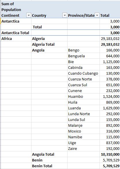
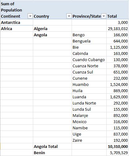
This pivot table looks awkward. The countries without provinces have a lone detail line, followed by a subtotal line with the exact same information. You can fix this by collapsing the single-item rows one at a time, but that’s time-consuming, and boring. Wouldn’t it be much more fun to write some code to hide pivot table single-item subtotals?

Pivot with single item subtotals

A year or so ago I did just that. In reviewing it for this post I cleaned it up and learned a few things about where it works and where it doesn’t. When I run it the result looks like this, with the duplicated population counts nicely hidden:

Pivot without single item subtotals

The heart of the code is this simple routine. You pass it a single PivotField and it hides the details for any item in that field that contains just one row:

Sub ProcessPivotField(pvtField As Excel.PivotField)
Dim ptItem As Excel.PivotItem

For Each ptItem In pvtField.PivotItems
    If ptItem.RecordCount > 1 Then
        ptItem.ShowDetail = True
    Else
        ptItem.ShowDetail = False
    End If
Next ptItem
End Sub

In my first version of this code I used ptItem.DataRange.Rows.Count. This caused errors with hidden items, because their DataRange is Nothing. With ptItem.RecordCount it just sails on through.

The main procedure checks whether the cursor is in a pivot table and a few things like that. It then calls a function that returns only the visible pivot table row and column fields:

Function GetPivotFieldNames(pvtTable As Excel.PivotTable) As String()
Dim PivotFieldNames() As String
Dim pvtField As Excel.PivotField
Dim i As Long
Dim PivotFieldsCount As Long

PivotFieldsCount = 0
With pvtTable
    ReDim Preserve PivotFieldNames(1 To .PivotFields.Count)
    For i = LBound(PivotFieldNames) To UBound(PivotFieldNames)
        Set pvtField = .PivotFields(i)
        If pvtField.Orientation = xlColumnField Or _
           pvtField.Orientation = xlRowField Then
            PivotFieldsCount = PivotFieldsCount + 1
            PivotFieldNames(PivotFieldsCount) = pvtField.Name
        End If
    Next i
End With
ReDim Preserve PivotFieldNames(1 To PivotFieldsCount)
GetPivotFieldNames = PivotFieldNames
End Function

The returned pivot fields are passed to a userform not unlike this one, except that it allows you to pick multiple items. That way you can collapse more than one field at a time. (I don’t show the code here, but you can get it all from the download link at the end.)

The form looks like this:

Collapsing single-item rows works great for lists like this one of continents, countries and provinces, because if a country has no subdivisions there’s no further detail to show. It’s just Iceland.

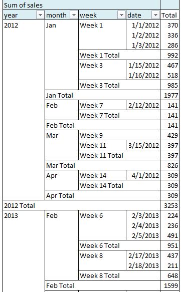
Where it doesn’t make as much sense is with something like sales by year, month, week and date:

Sales by week pivot

Even if you had sales in only one week in February, you’ll probably call it “week 6”, or “February 12 to 19”, or something. But when you collapse February that detail gets hidden.

Even more limiting is that you can’t collapse February for one year and leave it expanded for another. At least, I can’t find any way, either in VBA or in Excel. You either show a total for all your Februaries, or for none. In the example above it would be nice to hide the February 2012 total, but show it for 2013. If anybody knows a way to do that, please let us know.

To fool around with this for yourself you can download a workbook with a couple of sample pivots and the Single-Item Subtotal hider.

NOTE: I noticed a ways into this post that the population data is old. I tried to find something more recent, but didn’t come up with anything that had the provinces/states data. But it was nicely packaged in an Access database.

My Favorite F9 Trick

I’ll let you know right now this trick is not real fancy, or even best practice, but it is my favorite F9 trick so I’m sharing it. It basically changes a variable in a formula to a constant.

I’ve mentioned before the handiness of F9 when creating formulas. Highlighting part of a formula and pressing F9 evaluates just that part of the formula, converting it to its result. So if you have “=1+2+3” and you hit F9 with “2+3” selected, the formula becomes “=1 + 5.”

Before I get to the trick, here’s a longer F9 example.

Imagine you are generating emails from a list of addresses and attachments. One of the columns contains the names of the files to attach. There can be one or more attachment names per cell, separated by commas. There’s also a master list of all the attachments to be sent.

To verify whether all the attachments were included exactly one time, you can use an array formula like this in column E:

{=SUM(ISNUMBER(
FIND("," &  D3  & ",", ","  &  $B$2:$B$14  & ",")
)*1)=1}

If we highlight the 2nd row of that formula, in E3 and press F9 we get the following evaluation of the FIND section of the formula (with a few more #VALUE’s).

{#VALUE!;1;#VALUE!;#VALUE!;#VALUE!;#VAL …

FIND returns the position of the substring in the searched string, or #VALUE if the string isn’t found. The above tells us that the value in D3 is found once in B2:B14.

If you don’t already use F9, you should know that Ctrl-Z will undo the evaluation and return the formula to its formulaic state. You almost always want to do that, otherwise you’ll leave the hard-coded evaluation in the formula.

But not with my favorite F9 trick.

Even though it’s not a good practice in serious spreadsheets, sometimes I just want to hard-code a value into a formula. In these situations you can use F9 to insert the hard-coded value for you, and avoid typing errors. In this example, there’s a party with a randomized list of prizes for the guests.

F9 tip example

So, column C has your formula to randomize the prize distribution. But, for reasons only known to you, you’ve decided the grand prize of a new car must go to Bahijah, and you want to hard-code that into your formula.

You could just type IF(B2=”Bahijah“, but to avoid spelling errors you instead select B13.

=IF(B2=B13,"New Car",
INDEX(Sheet1!$E$2:$E$10,
RANDBETWEEN(1,COUNTA(Sheet1!$E$2:$E$10))))

You then highlight B13 and press F9 and the beginning of the formula becomes:

=IF(B2="Bahijah","New Car",

Below, I used a table so that the formula would change in every cell in column C, and you can see the car become Bahijah’s in one fell swoop.

F9 tip video