blog - Page 8 of 13 - yoursumbuddy

New Job!

Posted on February 2, 2014 by Doug Glancy

I recently said goodbye to my wonderful co-workers at Portland Public Schools and am now serving as a Report and System Developer for Kaiser Permanente. I’m excited to be part of Kaiser and impressed by its history and organization. Given the state of US health care, it will be an interesting place to work.

I’ll be doing less Excel and more SQL. And with luck my 18-mile round trip commute will give me the calves of a steroid-free Lance Armstrong. Or at least of my 7th-grade Spanish teacher, who had really big calves.

I’ve got a backlog of ideas for posts here, and just need the time and energy for them. A post often takes me upwards of 20 hours, sometimes a lot longer as I figure stuff out.

Whatever your endeavors in 2014, I wish you good luck.

Pivot Table Per-Item Color Scales

Posted on December 8, 2013 by Doug Glancy

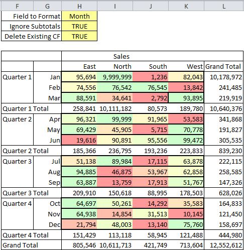
Let’s take another journey to the nexus of conditional formatting and pivot tables. My latest foray involved adding per-item color-scales to a pivot table, something like this, where the color scale is applied separately to each quarter:

You can see, for example, that the very high sales of $9,999,999 for January in Region 1 affect the color scale for the other cells in Quarter 1. However, the color scale within other quarters are unaffected, and a 99,999 value in Quarter 2 gets the same green that the much higher value did in Quarter 1.

Here’s another view with each month getting its own scale:

Finally, this shows icon sets by region. Notice that although they span each region for all months, the icon sets ignore the subtotals, which is often preferable:

My code allows you to include or include or ignore subtotals in each item’s color scale. I went about this a couple of ways before settling on the PivotTable.PivotSelect method. I learned about this method recently in a comment by Mike Alexander on one of Jeff Weir’s massive DDOE posts. I can’t find any good documentation, but in Excel 2007 forward you can do things like:

pvt.PivotSelect "'Row Grand Total'", xlDataOnly

Select a pivot table’s Row Grand Total area

pvt.PivotSelect "'Region'['East';Data]", xlDataOnly

Select the data rows for the East PivotItem of the Region PivotField

(There is a PivotSelect method in 2003, but these types of statements failed.)

It looks like PivotSelect is the VBA version of clicking, for example, a single subtotal in a pivot table and thereby selecting them all. I figured out the syntax by turning on the Macro Recorder and doing those types of selections:

I’m not crazy about using PivotSelect – I assume all that selecting will slow things down on big pivot tables. On the other hand it seems to work consistently. I had much more complicated code that worked most of the time, but only most.

Here’s the code, which runs in Excel 2007 on:

Sub PivotItemCF(pvtFieldToFormat As Excel.PivotField, IgnoreSubtotals As Boolean)
Dim pvt As Excel.PivotTable
Dim pvtItem As Excel.PivotItem
Dim pvtField As Excel.PivotField
Dim rngTest As Excel.Range

'Lots of selecting!
Application.ScreenUpdating = False

Set pvt = pvtFieldToFormat.Parent
With pvt
For Each pvtItem In pvtFieldToFormat.PivotItems
'A distressing number of possible errors from hidden items.
'If the item has no DataRange ignore it.
On Error Resume Next
Set rngTest = pvtItem.DataRange
If Err.Number = 0 Then
'Specify the Field name in case there are multiple items
'with the same name,for example from Grouping.
'Surround PivotItem names with single quotes in case they have spaces.
pvt.PivotSelect pvtFieldToFormat.Name & "['" & pvtItem.Name & "';Data;Total]", xlDataOnly
'Call routine that does the formatting
FormatRange Selection
End If
On Error GoTo 0
Next pvtItem

If IgnoreSubtotals Then
'Clear the FormatConditions from Row and Column fields
For Each pvtField In pvt.PivotFields
If pvtField.Orientation = xlRowField Or pvtField.Orientation = xlColumnField Then
'I can't figure a test for whether the subtotals are visible
'so just blindly firing away.
On Error Resume Next
.PivotSelect "'" & pvtField.Name & "'[All;Total]", xlDataOnly
If Err.Number = 0 Then
Selection.FormatConditions.Delete
End If
On Error GoTo 0
End If
Next pvtField
.PivotSelect "'Row Grand Total'", xlDataOnly
Selection.FormatConditions.Delete
.PivotSelect "'Column Grand Total'", xlDataOnly
Selection.FormatConditions.Delete
Else
End If
End With

Application.ScreenUpdating = True
End Sub

The FormatRange routine is just Macro Recorder code generated by selecting part of the pivot table and applying a color scale. You can do the same thing for data bars or icons.

In the sample workbook, the code is triggered by a WorkSheet_Change event that fires whenever one of the three yellow data validation cells is changed.

Curious Case of the Replaced Date Slash

Posted on November 15, 2013 by Doug Glancy

At my beloved workplace we’ve developed a fondness for slashes in institution names. If we’d been in charge, it would be Bachmann/Turner Overdrive, the Mason/Dixon line, Obsessive/Compulsive Disorder and well, you get the idea. Aesthetics aside, this causes problems when generating workbooks based on these names. Windows doesn’t like slashes in its file handles, because it uses them as path separators (except when it doesn’t, which is why you should use Application.PathSeparator in your code).

I recently wrote a little function to strip slashes and other shady characters out of file names and replace them with dashes, which don’t stick in Windows’ craw. Up until then, my co-worker was forced to do a search and replace on the offending monikers. In doing so she pointed out that the replace dialog mistakenly says it’s replacing all the slashes in the dates on the sheet as well, even though they remain in place.

For example, take a column like this, with one name and 1,048,574 dates:

And here it is with Excel proclaiming to have replaced 2,097,149 “/”s with “-“s, when clearly it only replaced the one. Silly old Excel!

I theorized that Excel was doing a two-step operation: first counting the slashes – including those in the dates – but then only replacing the non-date ones. I can certainly see myself doing something like that. We figured this was because Excel stores dates as numbers and the human/readable dates such like “11/15/2013” are just formats, and the slashes aren’t “really” there.

Turns out that’s wrong. I should have given Excel more credit. It really does replace the slashes if you ask it to. For example, try a find and replace with explanation points, or “bangs” as some folks call them. I get this:

What seems to happen with dashes is Excel recognizes them as date separators, but, at least on a computer with the slash set as the default date separator, it turns them right back into slashes. You can see this in it’s purest form by typing 11-15-2013 into a cell. It immediately converts the dashes, both in the formula bar and in the cell (at least if you’re using my laptop. I haven’t tested this extensively).

So it really is replacing all those millions of slashes with dashes. But then it converts them right back, without so much as a “by your leave.”

What’s confusing to me is that if I use a custom format like “yyyy.mm.dd” and try to replace the periods, Excel says there’s nothing to replace. That makes sense as the periods are just part of a format. But so are the slashes. What gives?

Speaking of dates, happy anniversary to my wonderful wife!

Filter as you type with FilterMatic!

Posted on October 27, 2013 by Doug Glancy

Whenever possible I employ lookups, crosswalks and whining to avoid correcting data by hand. Sometimes my best efforts fail, and I end up fixing lists one funky cell at a time. The horror! Happily I’ve created FilterMatic to ease the pain.

Say for instance, you’re giving a birthday party for a hundred or so of your oldest friends, all born on October 26. You’ve got this handy reference list of names, years of birth and notable accomplishment:

source:http://www.historyorb.com/today/birthdays.php

Meanwhile you’ve got another, very similar, list that calculates their age – with a lookup to the “year” column on the first list – so you can embarrass them by putting it on their place setting. The problem is some names are misspelled and you’re getting #N/A’s.

So you filter to just the #N/A’s and start to fix them. Wouldn’t it be nice if, as you fixed the errors, they were automatically filtered away? It’s true that in modern Excel tables you can do this with right-click>Filter>Re-Apply. But now with FilterMatic your corrections are instantly whisked from sight!

In the example below, I’m fixing the names, at first without FilterMatic running. After the third fix, I start it up. The first thing that happens is the filter is re-applied. After that the filter is re-applied with every change to the table and each fixed row is filtered away.

FilterMatic™ works on worksheet and table filters, re-applying them on the active sheet whenever you change a cell within a filtered area. And with FilterMatic™ there’s no confusing buttons or messy dropdowns. Just turn it on to start filtering! Close it when you’re done! But wait, there’s more! Download now and receive a free puppy!

Here’s the code:

Private WithEvents app As Excel.Application
Private WithEvents wsActive As Excel.Worksheet
'My ShowModal Property must be set to False

Private Sub UserForm_Activate()
Set app = Application
If Not ActiveSheet Is Nothing Then
Set wsActive = ActiveSheet
FilterMatic
End If
End Sub

Private Sub app_SheetActivate(ByVal Sh As Object)
Set Sh = wsActive
End Sub

Private Sub wsActive_Change(ByVal Target As Range)
FilterMatic
End Sub

Private Sub lblFilterMatic_DblClick(ByVal Cancel As MSForms.ReturnBoolean)
'apply changes by double-clicking the form
FilterMatic
End Sub

Sub FilterMatic()
Dim lo As Excel.ListObject

Set lo = Selection.ListObject
'if the selection overlaps a table
If Not lo Is Nothing Then
With lo
'Table is in filter mode
If .ShowAutoFilter Then
.AutoFilter.ApplyFilter
End If
End With
Else
'It will only re-apply a worksheet-level filter if
'there's no tables on the sheet.
With wsActive
'if sheet is filtered
If .FilterMode = True Then
'if the selection overlaps the worksheet's filtered area
If Not Intersect(Selection, .AutoFilter.Range) Is Nothing Then
.AutoFilter.ApplyFilter
End If
End If
End With
End If
End Sub

When the form is opened an application object is created. This object monitors all “SheetActivate” events in Excel and sets the activated worksheet to wsActive. There are three events that trigger the filtering code: opening the form, changing something in wsActive or clicking the label in the center of the form.

The FilterMatic sub checks for both ListObject and worksheet-level filters. If the selection at the time of the change intersects one, then that filter is updated. Note that if a listobject is found, it won’t go on to re-apply a worksheet filter. I tried that and couldn’t imagine a reasonable worksheet design that would have both filter types, and anyways the results were weird. Also note that if you change two listobjects at once, the filter would only be applied to one of them: whichever is the Selection.ListObject.

Here’s a workbook with the code and the lists.

And be sure to join the email list so you won’t miss my next exciting product: PivotMasher!

Get Unique Per-Row Values With RemoveDuplicates

Posted on October 10, 2013 by Doug Glancy

This post consists of two topics, both involving VBA’s RemoveDuplicates method. First I discuss an error and a shortcoming in the RemoveDuplicates documentation that have confounded myself and others. After those are cleared up I’ll show how to use RemoveDuplicates to return a two-dimensional array of unique items from a range containing one or more columns.

RemoveDuplicates was added to VBA (along with it’s front-end counterpart Data>Remove Duplicates) in Excel 2007. It’s very handy, allowing you to select one or more columns in a range and and winnow it down to the rows where the combined values of those columns are unique. It does this “in-place,” leaving other areas of the sheet intact.

RemoveDuplicates’ Columns Argument isn’t Really Optional

The Excel 2013 MSDN documentation describes the variant Columns argument as an optional “Array of indexes of the columns that contain the duplicate information. If nothing is passed then it assumes all columns contain duplicate information.” (my emphasis)

Later it gives an example of leaving out the Columns argument to remove duplicates from the entire range:

“The following code sample removes duplicates with all columns from a range.”

ActiveSheet.Range("A1:C100").RemoveDuplicates

However, testing reveals that the above code does nothing. This is confirmed by the perplexed comments of various forum visitors. In truth, you have to specify the columns variant array in all cases. The help example should look like this:

ActiveSheet.Range("A1:C100").RemoveDuplicates Columns:=Array(1,2,3)

If you want to base the removal on just some of the columns in a range, for example columns A and C, you do it like this:

ActiveSheet.Range("A1:C100").RemoveDuplicates Columns:=Array(1,3)

Using a Dynamic Columns Array

If you use RemoveDuplicates in code, there’s a good chance you’ll want to determine the array of column numbers at runtime and not hard-code them as above. As a simple test, I tried something like:

Dim ColumnsToCheck as Variant
ColumnsToCheck = Array(1,3)
ActiveSheet.Range("A1:C100").RemoveDuplicates Columns:=ColumnsToCheck

However this results in a Runtime Error ‘5’ – Invalid Procedure Call or Argument.

After looking around the web a while I found that the answer is to wrap ColumnsToCheck in parentheses, so the code becomes:

Dim ColumnsToCheck as Variant
ColumnsToCheck = Array(1,3)
ActiveSheet.Range("A1:C100").RemoveDuplicates Columns:=(ColumnsToCheck)

I know, from one of my all-time favorite DDOE posts that parentheses force evaluation of what’s inside them. Others on the web said that these parens “coerce” the evaluation of the array. I don’t really see how that applies here, so if you can explain why this works, please leave a comment.

One other note about the Columns variant array – it must be zero-based.

Unique Unique Per-Row Values Array Function

Once I’d sorted out the above points, I was able to use RemoveDuplicates as the basis of a function that returns a two-dimensional variant array containing the unique rows in a range. The range can consist of multiple columns that aren’t necessarily adjacent, as in this table of hometowns and sports of 2008 US Olympic athletes:

In the example above I want to return a variant array of all the unique combinations of the State and Sport fields. The specific use is for a worksheet splitter, where I prompt the user for one or two columns and the cycle through the array of unique combinations, creating a separate workbook for each combination.

The code is simple enough. It takes a range as it’s argument, for example the State and Sport fields above. It copies the range it to a worksheet in a newly added workbook. We then use RemoveDuplicates on the entire UsedRange of that new sheet. Because the columns are now contiguous the code can easily assign the modified range back to a variant array. The temporary workbook is then closed without saving.

Function GetUniqueRowValues(rng As Excel.Range) As Variant
Dim wbTemp As Excel.Workbook
Dim wsTemp As Excel.Worksheet
Dim ColNums As Variant
Dim i As Long

'if only one cell selected then can't pass to two-dimensional array
If rng.Cells.Count = 1 Then
'if the single cell is blank
If rng.Value = vbEmpty Then
Exit Function
Else
GetUniqueRowValues = rng.Value
Exit Function
End If
End If

Application.ScreenUpdating = False
Application.Calculation = xlCalculationManual
'create a temp workbook
'and copy range to it
Set wbTemp = Workbooks.Add
Set wsTemp = wbTemp.Worksheets(1)
With wsTemp
rng.Copy
'rng can consist of non-adjactent columns
'pasting to a new workbook results in a
'new range with only those columns
.Range("A1").PasteSpecial xlPasteValues
ReDim ColNums(0 To wsTemp.UsedRange.Columns.Count - 1)
'Create the array of column numbers for the
'RemoveDuplicates' Columns parameter
For i = LBound(ColNums) To UBound(ColNums)
ColNums(i) = i + 1
Next i
.UsedRange.RemoveDuplicates Columns:=(ColNums), Header:=xlGuess
'assign the values of the remaining,
'non-duplicated rows to the function result
GetUniqueRowValues = .UsedRange
End With
wbTemp.Close False
Application.ScreenUpdating = True
Application.Calculation = xlCalculationAutomatic
End Function

Note that is the original range was just one cell, the returned variant will not be an array. But you’d test for that before running this in the first place, wouldn’t you?

This code is fast for big ranges, handling over one million rows in less than five seconds on my laptop. On the other hand, it has to open and close a workbook, which takes part of a second and causes screen flicker. It’s a lot more flexible at least than my attempts to modify the Collection technique to handle large ranges with non-adjacent columns.

More Listbox Filtering With the Like Operator

Posted on September 12, 2013 by Doug Glancy

Since posting about filtering a listbox, I’ve been thinking a lot about VBA’s Like operator. I realized I could type in filters such as ‘[4-7]#‘ which matches two-digit numbers between 40 and 79. I raced to my computer to try it out, typed the opening bracket and was halted in my tracks:

It makes sense that a “[” without a “]” is untenable in a Like pattern. It needs the closing bracket to mark the end of the character set. On the other hand, a single “]” is legal and just stands for itself. You can match a left bracket by putting brackets around it, so the following expression in the Immediate Window yields True:

? "[" Like "[[]"

I set to creating a function that would detect the invalid left bracket. I tried testing whether there were more left than right brackets, but since you can have two left ones in a row, and as many right ones as you want, that wouldn’t fly. To avoid a complicated set of tests, I turned to the VBA standby of attempting something inside of On Error statements, something whose failure yields specific and helpful information, like “hey that’s an invalid pattern.”

Here was the first attempt, which seemed to do the trick:

Function ValidLikePattern(LikePattern As String) As Boolean
Dim temp As Boolean
On Error Resume Next
temp = ("A" Like LikePattern)
If Err.Number = 0 Then
ValidLikePattern = True
End If
On Error GoTo 0
End Function

You pass it a pattern and it tests it against the simplest possible string – “A”. My assumption was the test would either pass, if there was no left bracket, or fail if there was. I was wrong on two counts.

The first is that Like actually has three possible outcomes: True, False or Null. It returns Null if either the string being compared or the pattern is an empty string.

Much more important to my function, Like is lazy. It only tests as far as needed. So, while this returns an “Invalid pattern string” message:

? "A" Like "["

This doesn’t:

? "A" Like "A["

It just returns False. I guess Like compares the first characters, sees they match and checks whether the next one is an asterisk, the only character that could match at this point. Since it’s not, Like says “whatever” and quits, ignoring the left bracket’s tenuous status.

I could fix the function – kind of – by using a really long string in place of “A” and force Like to look harder. Instead I surrounded LikePattern in asterisks:

temp = ("A" Like "*" & LikePattern & "*")

This says there could be an infinite number of characters at the beginning of the pattern, so Like needs to be thorough and compare all the way through. I suppose this slows the code. I also guess I don’t need the “*” at the end. At any rate, I can now type a left bracket into the filter textbox without an error:

I updated the sample workbook from the ListBox Filter With WildCards post. It now calls the ValidLikePattern function at the beginning of the main loop. If the pattern isn’t valid, the loop is exited and the filtering stays the same until the next change in the filter textbox. Here’s the updated download.

Help Me Test Table Viewer

As I mentioned at the end of that post, I’m incorporating this logic and a bunch of features into a Table Viewer addin. I think it’s even more “freakin’ awesome” than MenuRighter. I’ve been using it every day. I just added the ability to specify exact matches, “contains”, “begins with”, etc. If you’d like to help me test it, please leave a comment or use the contact form to let me know. Or wait for my next post.

Camera Tool – Now With 33% More Picture

Posted on September 11, 2013 by Doug Glancy

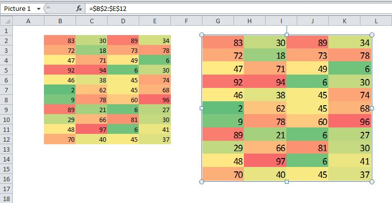
I’ve posted before about Excel’s handy camera tool. I don’t use it much, but I have one monster report that relies on it extensively. It contains code that uses the Shape object’s ScaleWidth method. I went to run the report yesterday and all my camera-generated-pictures got bigger. For reasons lost in the murk of time, I was setting the pictures’ ScaleWidth’s to 1, which made them adjust nicely when the range they point at changes size.

Anyways, all of a sudden the pictures got bigger when the code ran. So I came home and reproduced it on a different computer, without code. Sure enough, the same thing. Below I list a couple simple steps to demo the problem. Both machines I tested were Windows 7, Office 2010 SP2 with the latest patches on both:

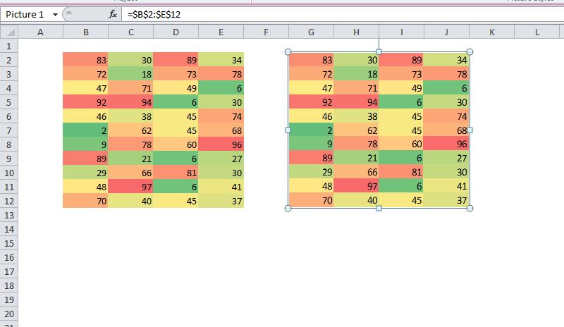
First, take a picture of a range:

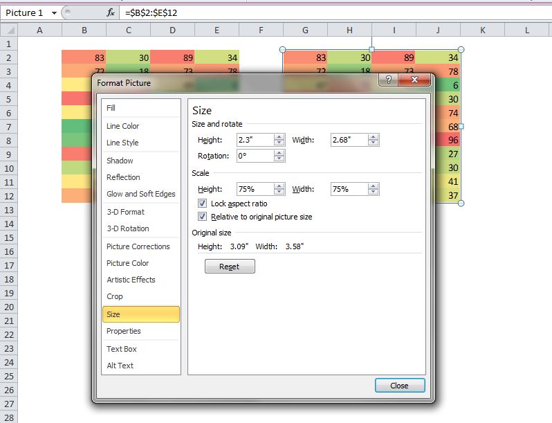
Second, right-click and choose Size and Properties (or Alt-JP-O for the mouse-averse). Note that the height and width are listed as 75% and the original size is listed as bigger than the current size:

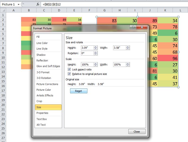
Finally, hit the Reset button and see your picture magically grow! Note that the height and width are now shown as 100% and we’ve achieved the “Original Size”:

In my limited testing it seems to always be a factor of 75%. So now my code uses ScaleWidth 0.75. I set it as a Const, because talk about a magic number!

Anybody know the cure for this? I searched, and though the camera tool has a fairly rich history of bugs, I didn’t see this behavior mentioned anywhere.

P.S. I know that it’s really more than 33%.

ListBox Filter With Wildcards and Unique Values

Posted on September 2, 2013 by Doug Glancy

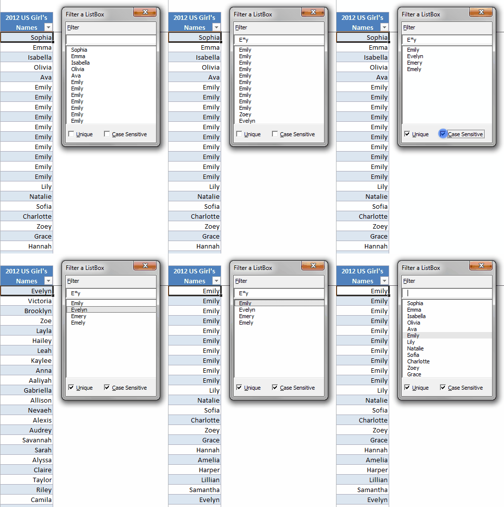
This post demonstrates a simple setup to filter a userform listbox as you type into a textbox. The filter uses VBA’s Like operator to pick up matches anywhere within the string. For example, typing “ursumb” matches to “yousumbuddy.” The Like operator allows wildcards, so “/*/201?” matches all dates from 2010 onwards. Like is also case-sensitive, so it can filter by case, or not, as specified. In addition the code uses the tried and true Collection method to allow filtering by unique items.

So, with this list of most popular US girls’ names for 2012 (modified in favor of “Emily”) you can filter and then add Unique and Case Sensitive filters. Note that clicking a name takes you to that row in the table:

Nice, isn’t it? Here’s the main routine, which gets called whenever the text in the filter textbox changes or one of the checkboxes is clicked:

Sub ResetFilter()
Dim rngTableCol As Excel.Range
Dim varTableCol As Variant
Dim RowCount As Long
Dim collUnique As Collection
Dim FilteredRows() As String
Dim i As Long
Dim ArrCount As Long
Dim FilterPattern As String
Dim UniqueValuesOnly As Boolean
Dim UniqueConstraint As Boolean
Dim CaseSensitive As Boolean

'the asterisks make it match anywhere within the string
FilterPattern = "*" & Me.txtFilter.Text & "*"
UniqueValuesOnly = Me.chkUnique.Value
CaseSensitive = Me.chkCaseSensitive

'used only if UniqueValuesOnly is true
Set collUnique = New Collection
Set rngTableCol = loActive.ListColumns(1).DataBodyRange
'note that Transpose won't work with > 65536 rows
varTableCol = Application.WorksheetFunction.Transpose(rngTableCol.Value)
RowCount = UBound(varTableCol)
ReDim FilteredRows(1 To 2, 1 To RowCount)
For i = 1 To RowCount
If UniqueValuesOnly Then
On Error Resume Next
'reset for this loop iteration
UniqueConstraint = False
'Add fails if key isn't UniqueValuesOnly
collUnique.Add Item:="test", Key:=CStr(varTableCol(i))
If Err.Number <> 0 Then
UniqueConstraint = True
End If
On Error GoTo 0
End If
'True if UniqueValuesOnly is false or if
'UniqueValuesOnly is True and this is the
'first occurrence of the item
If Not UniqueConstraint Then
'Like operator is case sensitive,
'so need to use LCase if not CaseSensitive
If (Not CaseSensitive And LCase(varTableCol(i)) Like LCase(FilterPattern)) _
Or (CaseSensitive And varTableCol(i) Like FilterPattern) Then
'add to array if ListBox item matches filter
ArrCount = ArrCount + 1
'there's a hidden ListBox column that stores the record num
FilteredRows(1, ArrCount) = i
FilteredRows(2, ArrCount) = varTableCol(i)
End If
End If
Next i
If ArrCount > 0 Then
'delete empty array items
'a ListBox cannot contain more than 65536 items
ReDim Preserve FilteredRows(1 To 2, 1 To Application.WorksheetFunction.Min(ArrCount, 65536))
Else
're-initialize the array
Erase FilteredRows
End If
If ArrCount > 1 Then
Me.lstDetail.List = Application.WorksheetFunction.Transpose(FilteredRows)
Else
Me.lstDetail.Clear
'have to add separately if just one match
'or we get two rows, not two columns, in ListBox
If ArrCount = 1 Then
Me.lstDetail.AddItem FilteredRows(1, 1)
Me.lstDetail.List(0, 1) = FilteredRows(2, 1)
End If
End If
End Sub

This routine takes advantage of the fact that Collection keys must be unique. If “Unique” is checked on the form, we test each value before adding it to the ListBox’s array.

The FilterPattern string has asterisks at the beginning and end. This is why the filter matches if it’s found anywhere within a table item.

In addition to the girl’s name, an array item also holds the record number for that name. This is used in another subroutine that activates the table row when the listbox selection changes:

Private Sub lstDetail_Change()
GoToRow
End Sub

Sub GoToRow()
If Me.lstDetail.ListCount > 0 Then
Application.Goto loActive.ListRows(Me.lstDetail.Value).Range.Cells(1), True
End If
End Sub

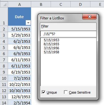
Here’s how it looks when filtering dates:

The speed is quite reasonable for tables with less than 10,000 items. Above that it gets slow, but is still usable all the way up to the limit of 65,536 listbox items. Yikes!

Here’s a workbook with all the code and the name and date tables to fool around with.

An Invitation

I’ve expanded this concept into a full-fledged Table Viewer. I’ve been using it in its alpha state and it’s quite handy for zipping around a big table. Along with the features here, it handles multiple columns, allows you to view only visible rows, and some other stuff. If anybody is interested in testing it out, leave a comment here or use the contact form.

Prompt to Add New Items to ComboBox or Data Validation

Posted on June 2, 2013 by Doug Glancy

Microsoft Access ComboBoxes have a handy NotinList event which allow you to check whether a value entered in a combobox is already in its list. If it’s not you can ask the user whether to add it. This post shows how to mimic that functionality in a combobox on a VBA userform. I also show how to do the same thing with a data validation list.

Creating a ComboBox NotInList Event

The key to doing this is checking the value of the ComboBox’s “MatchFound” property in its Exit event. If no match is found, we ask the user whether to add the item to the list of valid items (hats in this case). If the answer is “Yes” then a row with the hat is added to the table. If not, we clear the combobox and keep the focus on it. You can see this in action in the video above.

Here’s the code for the combobox’s Exit event:

Private Sub cboHats_Exit(ByVal Cancel As MSForms.ReturnBoolean)
Dim loValidationSource As Excel.ListObject
Dim loRow As Excel.ListRow

'the Table with the list of valid hats
Set loValidationSource = wsTables.ListObjects("tblValidationSource")
With Me.cboHats
'We're only interested if these aren't true
If .MatchFound Or .Value = "" Or .Value = STARTING_VALUE Then
Exit Sub
End If
'If the hat entered isn't in list, prompt to add it
If MsgBox(.Value & " is not in the list. Add it?", vbYesNo + vbDefaultButton2 + vbQuestion) = vbYes Then
Set loRow = loValidationSource.ListRows.Add
loRow.Range.Cells(1).Value = .Value
SortSourceTable
RefreshComboList
Else
'if "no", keep focus on the ComboBox and set it's value to "Choose a hat"
Cancel = True
Me.cboHats.Value = STARTING_VALUE
End If
End With
End Sub

One important thing is that the combobox’s “MatchRequired” property must be set to False (which is the default). Otherwise the Exit will be preempted by an “Invalid Property Value” message from Excel.

Creating a Data Validation NotInList Event

As with the combobox version, we use an event to prompt the user whether to add an item that’s not in the list. This time we use our own “MatchFound” function to check against the data validation’s source list. Similar to setting the “Match Required” combobox property to False, the data validation version requires that the “Show error alert after invalid data is entered” is unchecked in the data validation setup dialog. This is obviously not the default:

Since I’m working in Excel 2010, I’ve created a single-column table (listobject) to hold the valid items. I then simply pointed the data validation’s Source property at the column, excluding the header. Because the source is in a table, it’s dynamic – it adjusts when you add or remove items from the column. No dynamic ranges are required, just select the cells:

Here’s the code from the ThisWorkbook module, which contains the Workbook_SheetChange event and the MatchFound function:

Private Sub Workbook_SheetChange(ByVal Sh As Object, ByVal Target As Range)
Dim cell As Excel.Range
Dim loValidationSource As Excel.ListObject
Dim loHatCollection As Excel.ListObject
Dim loRow As Excel.ListRow

'wsTables is the sheet's CodeName
If Not Sh Is wsTables Then
Exit Sub
End If
Set loValidationSource = wsTables.ListObjects("tblValidationSource")
Set loHatCollection = wsTables.ListObjects("tblHatCollection")
'only continue if change is in column with data validation
If Intersect(Target, loHatCollection.ListColumns("Hat Type").DataBodyRange) Is Nothing Then
Exit Sub
End If
With Intersect(Target, loHatCollection.ListColumns("Hat Type").DataBodyRange)
For Each cell In .Cells
If MatchFound(cell.Value) = False And cell.Value <> "" Then
If MsgBox(cell.Value & " is not in the list. Add it?", vbYesNo + vbDefaultButton2 + vbQuestion) = vbYes Then
Set loRow = loValidationSource.ListRows.Add
loRow.Range.Cells(1).Value = cell.Value2
Else
cell.ClearContents
End If
End If
Next cell
End With
SortSourceTable
End Sub

Function MatchFound(ValueToCheck As Variant) As Boolean
Dim loValidationSource As Excel.ListObject
Dim ValidationList As Excel.Range

Set loValidationSource = wsTables.ListObjects("tblValidationSource")
Set ValidationList = loValidationSource.ListColumns("Hats Validation List").DataBodyRange
MatchFound = Application.WorksheetFunction.CountIf(ValidationList, ValueToCheck) > 0
End Function

And here’s what it looks like in action:

The Sort object – Excel 2007 Onwards

My code uses VBA’s Sort object, which appeared in Excel 2007. I like the way it works. You add Sort Fields, just as you do in the user interface, and then apply the sort when needed. If you are using Excel 2003 or earlier you’d need to re-write the two sorting procedures to work with your version.

Also, if you are using Excel 2003 or earlier, see this Contextures post for a non-table way of automatically adding items to a data validation list. You could easily add the code to prompt the user whether to do so.

Download

Here’s a workbook with all the code for both versions.

Filter Pivot Tables Using Source Data Helper Columns

Posted on May 19, 2013 by Doug Glancy

When working with pivot tables you often need to filter out certain items. You can of course do this directly in the fields’ filter dropdowns, and often that’s good enough. But if you change the filters repeatedly this can be tedious and error-prone. For this reason, and to make my workbooks more flexible and maintainable, I often add helper columns to the source data. This post explains three types of source data helper columns that I use to filter pivot tables.

The live workbook below contains a simple data set of All-Star baseball games, where they were held, and which league won. It also contains three helper columns, each using a different method to determine the rows included in the pivot table. All three techniques refer to tables that spell out the criteria for inclusion.

(You can switch tabs, edit cells and refresh pivot tables. Reloading this page reverts it to its starting state. Note the buttons for downloading or opening in a full web page.)

You can click into the formulas in the helper columns and see that they are referring to tables – a different one for each column. Each formula uses a COUNTIF or COUNTIFS function to determine if the venue for that row meets certain criteria.

When you click on the “pivot and helper tables” tab you’ll see the pivot table on the left and the three helper tables on the right. The pivot table has a report filter for each of the three helper columns. Note that the report filters, table headers and helper columns are color-coded to show which ones go together.

Okay, let’s look at the three methods in order.

Table Containing Only Values to Include

Back on the data tab, the helper column “Venue In Table” looks at the first table, the one titled “Venues to Include”. The formula is a simple one:

=COUNTIF(tblVenuesToInclude[Venues to Include],[@Venue])>0

It returns TRUE if the ballpark for that row is found in the table. Its report filter is already set to TRUE in the pivot table, so you can test it by adding or deleting a stadium name in the table, right-clicking the pivot table and clicking “refresh”.

Table With All Values and an “Include” column

The second helper column/table pair are very similar, but instead of a table listing only the baseball fields you want included, you list all of them and add another column that contains TRUE if the ballpark should be included. I might use this method if I had a table with all the venues that I was already using for another purpose:

=COUNTIFS(tblVenuesIncludeCol[Venue],[@Venue],tblVenuesIncludeCol[Include],TRUE)>0

The COUNTIFS formula checks both the Venue and the Include columns. (You can use a SUMPRODUCT formula if you’re using Excel 2003 or earlier). You can test this formula by changing its report filter to TRUE and then changing the values in the Include column of the 2nd table.

Table Containing Words to Look For

The final helper column is “Venue Word in Table”. It looks into the “Word to Find” table and uses a COUNTIF array formula that searches the venue’s name for words from the table. Changing the report filter to TRUE will find the Kingdome, Polo Grounds and any park whose name contains “field”.

Here’s the formula, entered with Ctrl-Shift-Enter:

{=MAX(COUNTIF([@Venue],"*" & tblWordToFind[Word to Find] & "*"))>0}

This formula takes advantage of the ability to use wildcards in COUNTIF functions, by putting asterisks before and after the table column reference. Being an array formula, it tests the venue name against each word in the “Word to Find” table. The 1934 data row returns TRUE because “Polo Grounds” contains the word “polo”, which is in the table.

If we use the F9 key to successively evaluate parts of the function it looks like this:

=MAX(COUNTIF([@Venue],"*" & tblWordToFind[Word to Find] & "*"))>0

=MAX(COUNTIF([@Venue],"*" & {"king";"polo";"field"} & "*"))>0

=MAX(COUNTIF("Polo Grounds","*" & {"king";"polo";"field"} & "*"))>0

=MAX({0;1;0})>0

=1>0

TRUE

One final note: In actual practice, I always put the helper tables on a separate sheet, not next to the pivot table as done here. Expanding pivot tables, among other things, makes this layout impractical in real use.