goofy code

The other day I needed to increment some footnotes for a document that gets published yearly. The footnotes look something like:

(8,11)

I needed to increment them all by three and there are a few pages, so of course I wrote some VBA. The line that prompted this post removes the left and right parentheses, then Splits the remaining string with comma as the delimiter, and assigns the resulting array to a variant. Here it is:

 SplitCell = Split(Replace(Replace(cell.Value2, ")", ""), "(", ""), ",")

I admit I’m easily amused, but that is some funny looking code.

Re-Apply Pivot Table Conditional Formatting

I often use conditional formatting in pivot tables, often to add banding to detail rows and highlights to total rows.  I like conditional formatting in XL 2010 for the most part, but sometimes it’s persnickety.  It seems to change its mind from day-to-day about what’s allowed.

One well-known problem is that if you apply conditional formatting to both your row fields and the data items, like this:
pivot table with intact conditional formatting

and then refresh it, the formatting is wiped from the data (values) area, as shown below:

There are a couple of ways to fix this.  One is to specifically apply the formats to the values area(s), a new feature as of Excel 2007.  Conditional formats added this way aren’t cleared by pivot table refreshes:
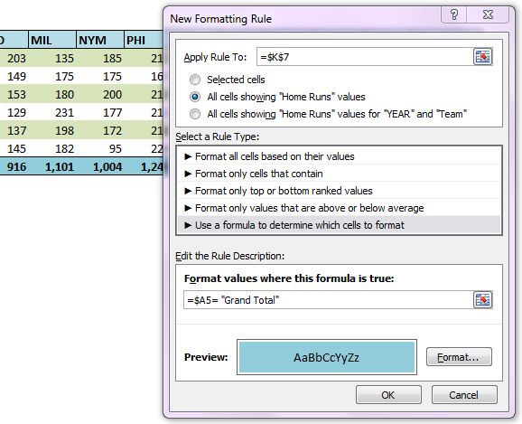
apply CF to data area

This works fairly well as long as your data area only includes one values field, but if you are pivoting on multiple values fields, you’ll have to add the rule for each one.  And you can’t specify row fields in this dialog, so you’ll have define the formats again for those areas.  And if you alter the formats you’ll have to do it all again.

For these reasons I’d rather just apply the conditional formatting to the row headings and the values area in one fell swoop.  But I don’t want to visit the condtional formatting dialog to re-expand the range each time a pivot table is refreshed.

So, I wrote the code below to expand the condtional formatting from the first row label cell into all the row label and data area cells:

Sub Extend_Pivot_CF_To_Data_Area()
Dim pvtTable As Excel.PivotTable
Dim rngTarget As Excel.Range
Dim rngSource As Excel.Range
Dim i As Long

'check for inapplicable situations
If ActiveSheet Is Nothing Then
    MsgBox ("No active worksheet.")
    Exit Sub
End If
On Error Resume Next
Set pvtTable = ActiveSheet.PivotTables(ActiveCell.PivotTable.Name)
If Err.Number = 1004 Then
    MsgBox "The cursor needs to be in a pivot table"
    Exit Sub
End If
On Error GoTo 0

With pvtTable
    'format conditions will be applied to row headers and values areas
    Set rngTarget = Intersect(.DataBodyRange.EntireRow, .TableRange1)
    'set the format condition's source to the first cell in the row area
    Set rngSource = rngTarget.Cells(1)
    With rngSource.FormatConditions
        For i = 1 To .Count
            'reset each format condition's range to row header and values areas
            .Item(i).ModifyAppliesToRange rngTarget
        Next i
    End With

    'display isn't always refreshed otherwise
    Application.ScreenUpdating = True
End With
End Sub

The key to this code is the ModifyAppliesToRange method of each FormatCondtion. This code identifies the first cell of the row label range and loops through each format condition in that cell and re-applies it to the range formed by the intersection of the row label range and the values range, i.e., the banded area in the first image above.

This method relies on all the conditional formatting you want to re-apply being in that first row labels cell. In cases where the conditional formatting might not apply to the leftmost row label, I’ve still applied it to that column, but modified the condition to check which column it’s in.

This function can be modified and called from a SheetPivotTableUpdate event, so when users or code updates a pivot table it re-applies automatically. I’ve also added this macro to the Pivot Table Context Menu and some days it gets used a lot.

Building A Workbook Table Class

Tables in Excel 2010 are powerful tools that help me hugely in my work as a data analyst. I use them every day.

Excel 2003 tables (called lists) were worksheet-level objects.  You could give two tables the same name if they were on different sheets, and not hear a word of complaint out of Excel.  In XL 2010 they are workbook-level objects, so you can use any given table name only once in a workbook.  They are also workbook-level in that you can reference a table from any formula in any sheet just by beginning to type its name, same as with a function or a named range.

In VBA, tables, or listobjects, as they continue to be known, are still worksheet-level objects.  You can declare a Worksheet.Listobject but not a Workbook.Listobject.

I’m working on a project where I wanted a Workbook.Listobject class, so I built one.  To do so, I created a new class called cWorkbookTables and added the following code:

Dim m_wb As Excel.Workbook
Dim m_Tables As Collection

Public Property Get NewEnum() As IUnknown
'the following line, added in a text editor,
'creates the ability to cycle through the items with For Each
'Attribute NewEnum.VB_UserMemId = -4
Set NewEnum = m_Tables.[_NewEnum]
End Property

Public Function Initialize(WbWithTables As Excel.Workbook)
Set m_wb = WbWithTables
Refresh
End Function

Public Sub Refresh()
Dim ws As Excel.Worksheet
Dim lo As Excel.ListObject

Set m_Tables = New Collection
For Each ws In m_wb.Worksheets
  For Each lo In ws.ListObjects
    m_Tables.Add lo, lo.Name
  Next lo
Next ws
End Sub

Public Property Get Item(Index As Variant) As Excel.ListObject
'the following line, added in a text editor,
'sets Item as the default property of the class
'Attribute Item.VB_UserMemId = 0
Set Item = m_Tables(Index)
End Property

Public Property Get Count()
Count = m_Tables.Count
End Property

Property Get Exists(Index As Variant) As Boolean
Dim test As Variant
On Error Resume Next
Set test = m_Tables(Index)
Exists = Err.Number = 0
End Property

Note that the code above includes two lines that have to be added in a text editor. The commented lines set the default property for the class, which is Item, and add the ability to enumerate through the class members in a For Each loop. The processes for adding these very nice features are described in various places on the web, including these instructions at Chip Pearson’s site.

In the same workbook I added two tables and ran the code below in a regular module:

Sub TestTableClass()
Dim clsTables As cWorkbookTables
Dim lo As Excel.ListObject
Dim i As Long

Set clsTables = New cWorkbookTables
With clsTables
  .Initialize ThisWorkbook
  Debug.Print "Number of tables in workbook: " & .Count
  For i = 1 To .Count
    Debug.Print "clsTables(" & i & ") name: " & .Item(i).Name
  Next i
  For Each lo In clsTables
    Debug.Print lo.Name & " " & lo.DataBodyRange.Address
  Next lo
End With
Debug.Print "There is a Table1: " & clsTables.Exists("Table1")
Debug.Print "There is a Table3: " & clsTables.Exists("Table3")
End Sub

The results in the Immediate Window look like this:

Number of tables in workbook: 2
clsTables(1) name: Table1
clsTables(2) name: Table2
Table1 $A$2:$B$4
Table2 $A$2:$B$4
There is a Table1: True
There is a Table3: False

For the reasons mentioned at the beginning of this post, this class only works in XL 2007 and 2010.

Workbook Tables Class Intellisense