VBA Archives - Page 7 of 8

Copy Table Data While Not Breaking References

Posted on April 5, 2012 by Doug Glancy

I’ve mentioned before I’m a big fan of tables in Excel 2010. One way I use them is in models, where each table represents a different scenario. The models let users create new scenarios, based either on an existing one or a blank template. Each version is stored in a table in its own worksheet. These tables always have the same fields (columns) but the values in the variable fields are different. The number of rows can differ from table to table.

I often want to copy, in VBA, the contents from a “source” to a “target” table. If I just copy the whole thing, the target table will be overwritten and renamed – something like “tblSource1” (adding a “1” to the source table name). That breaks any formulas referring to “tblTarget.” They’ll show a #REF error because they can’t find “tblTarget.” So I need code that copies the table data from tblSource to tblTarget without completely replacing tblTarget.

I’ve been writing code on a case-by-case basis, but thought that I’d generalize it a bit more. In addition to keeping the table’s identity intact, it should copy the source’s totals row if there is one, and turn off the target’s total row if there isn’t. The number of rows should increase or decrease to match the source. And, although I’ve only ever copied tables as values, I want the option to copy formulas.

I thought about dealing with a different number of columns but, at least in my uses so far, that shouldn’t happen. If I ever do try to accommodate models with changing numbers of fields, I think I’d do some testing before ever calling this code, and adjust the headers in another procedure.

So here’s what I came up with:

Sub CopyTableData(loSource As Excel.ListObject, loTarget As Excel.ListObject, Optional CopyFormulas As Boolean = False)
Dim FormulaCells As Excel.Range

With loTarget
If .DataBodyRange.Rows.Count <> loSource.DataBodyRange.Rows.Count Then
'have to clear target otherwise old table content may be outside new table
.DataBodyRange.Cells.Clear
'set target rows count to source rows count
.Resize .Range.Cells(1).Resize(loSource.HeaderRowRange.Rows.Count + _
loSource.DataBodyRange.Rows.Count, loSource.Range.Columns.Count)
End If
loSource.DataBodyRange.Copy Destination:=.DataBodyRange.Cells(1)
If CopyFormulas Then
On Error Resume Next
'any formulas?
Set FormulaCells = .DataBodyRange.SpecialCells(xlCellTypeFormulas)
On Error GoTo 0
'if yes, then replace any references to source table with target
If Not FormulaCells Is Nothing Then
FormulaCells.Replace what:=loSource.Name, replacement:=.Name, lookat:=xlPart
End If
Else
.DataBodyRange.Value2 = .DataBodyRange.Value2
End If

'turn target Totals row on or off to match Source
If loSource.ShowTotals Then
.ShowTotals = True
loSource.TotalsRowRange.Copy Destination:=.TotalsRowRange
Else
.ShowTotals = False
End If
End With

End Sub

One thing I learned is that there are two Resizes in a table (listobject). The first type, the Range property, was familiar, e.g.,

Range("A1").Resize(20,1)

… which yields a range object whose address is A1:A20.

The second is the Listobject.Resize method, which allows you to modify a table’s range, e.g.,

loTarget.Resize(Range("A1:F20")

which will change loTarget’s range to A1:F20.

Both of these types of Resizes are used in the code above, in the same line, happily enough.

Data Normalizer

Posted on March 28, 2012 by Doug Glancy

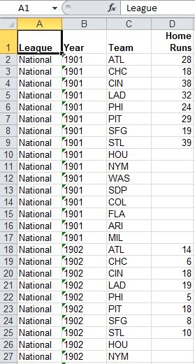
Sometimes I get data like this…

that needs to be like this…

The goal here is to roll up all the home runs into one, much longer, column. The data will then be pivot-worthy.

Generally, I need to keep one or more leftmost column headers, in this case “League” and “Year.” I need a new column to describe the rolled-up category (“Team”) and one for the data itself (“Home Runs”). I’ve written code a couple of times to handle specific cases and thought I’d try to generalize it. Here’s the result:

'Arguments
'List: The range to be normalized.
'RepeatingColsCount: The number of columns, starting with the leftmost,
' whose headings remain the same.
'NormalizedColHeader: The column header for the rolled-up category.
'DataColHeader: The column header for the normalized data.
'NewWorkbook: Put the sheet with the data in a new workbook?
'
'NOTE: The data must be in a contiguous range and the
'rows that will be repeated must be to the left,
'with the rows to be normalized to the right.

Sub NormalizeList(List As Excel.Range, RepeatingColsCount As Long, _
NormalizedColHeader As String, DataColHeader As String, _
Optional NewWorkbook As Boolean = False)

Dim FirstNormalizingCol As Long, NormalizingColsCount As Long
Dim ColsToRepeat As Excel.Range, ColsToNormalize As Excel.Range
Dim NormalizedRowsCount As Long
Dim RepeatingList() As String
Dim NormalizedList() As Variant
Dim ListIndex As Long, i As Long, j As Long
Dim wbSource As Excel.Workbook, wbTarget As Excel.Workbook
Dim wsTarget As Excel.Worksheet

With List
'If the normalized list won't fit, you must quit.
If .Rows.Count * (.Columns.Count - RepeatingColsCount) > .Parent.Rows.Count Then
MsgBox "The normalized list will be too many rows.", _
vbExclamation + vbOKOnly, "Sorry"
Exit Sub
End If

'You have the range to be normalized and the count of leftmost rows to be repeated.
'This section uses those arguments to set the two ranges to parse
'and the two corresponding arrays to fill
FirstNormalizingCol = RepeatingColsCount + 1
NormalizingColsCount = .Columns.Count - RepeatingColsCount
Set ColsToRepeat = .Cells(1).Resize(.Rows.Count, RepeatingColsCount)
Set ColsToNormalize = .Cells(1, FirstNormalizingCol).Resize(.Rows.Count, NormalizingColsCount)
NormalizedRowsCount = ColsToNormalize.Columns.Count * .Rows.Count
ReDim RepeatingList(1 To NormalizedRowsCount, 1 To RepeatingColsCount)
ReDim NormalizedList(1 To NormalizedRowsCount, 1 To 2)
End With

'Fill in every i elements of the repeating array with the repeating row labels.
For i = 1 To NormalizedRowsCount Step NormalizingColsCount
ListIndex = ListIndex + 1
For j = 1 To RepeatingColsCount
RepeatingList(i, j) = List.Cells(ListIndex, j).Value2
Next j
Next i

'We stepped over most rows above, so fill in other repeating array elements.
For i = 1 To NormalizedRowsCount
For j = 1 To RepeatingColsCount
If RepeatingList(i, j) = "" Then
RepeatingList(i, j) = RepeatingList(i - 1, j)
End If
Next j
Next i

'Fill in each element of the first dimension of the normalizing array
'with the former column header (which is now another row label) and the data.
With ColsToNormalize
For i = 1 To .Rows.Count
For j = 1 To .Columns.Count
NormalizedList(((i - 1) * NormalizingColsCount) + j, 1) = .Cells(1, j)
NormalizedList(((i - 1) * NormalizingColsCount) + j, 2) = .Cells(i, j)
Next j
Next i
End With

'Put the normal data in the same workbook, or a new one.
If NewWorkbook Then
Set wbTarget = Workbooks.Add
Set wsTarget = wbTarget.Worksheets(1)
Else
Set wbSource = List.Parent.Parent
With wbSource.Worksheets
Set wsTarget = .Add(after:=.Item(.Count))
End With
End If

With wsTarget
'Put the data from the two arrays in the new worksheet.
.Range("A1").Resize(NormalizedRowsCount, RepeatingColsCount) = RepeatingList
.Cells(1, FirstNormalizingCol).Resize(NormalizedRowsCount, 2) = NormalizedList

'At this point there will be repeated header rows, so delete all but one.
.Range("1:" & NormalizingColsCount - 1).EntireRow.Delete

'Add the headers for the new label column and the data column.
.Cells(1, FirstNormalizingCol).Value = NormalizedColHeader
.Cells(1, FirstNormalizingCol + 1).Value = DataColHeader
End With
End Sub

You’d call it like this:

Sub TestIt()
NormalizeList ActiveSheet.UsedRange, 2, "Team", "Home Runs", False
End Sub

It runs pretty fast. The sample sheet above – 109 years of data by 16 teams – completes instantly. 3,000 rows completes in a couple of seconds.

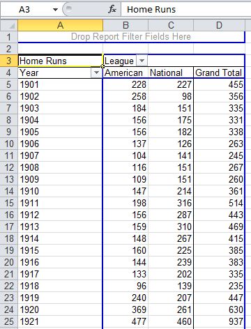
If I also run the routine on some American League data and put all the new rows in one sheet (with the same column headers) I can generate a pivot table that looks like this, which I couldn’t have done with the original data:

You can download a zip file with a .xls workbook that contains the data and code. Just click on the “normalize” button.

A Flexible VBA Chooser Form

Posted on March 20, 2012 by Doug Glancy

Fairly often in VBA code I need to offer the user a list and have them make a choice, like picking which open workbook to do something to. I created a function and a userform to handle these situations. (Around the house, I call the form “ChooserForm” but it’s given name is “frmChooser.”) The function takes an array of choices and a caption as its arguments. The function loads frmChooser and passes it the string array and the caption. When the user makes a choice and clicks OK the function returns the choice to the calling routine.

Let’s look at how it works, starting from the inside out (by which I mean with the userform):

The frmChooser UserForm

Private mboolClosedWithOk As Boolean
Private mChoiceList() As String

Public Property Let ChoiceList(PassedList() As String)
mChoiceList() = PassedList()
End Property

Private Sub UserForm_Activate()
With Me.cboChooser
.List = mChoiceList()
.ListIndex = 0
End With
End Sub

Public Property Get ChoiceValue() As String
ChoiceValue = Me.cboChooser.Value
End Property

Private Sub cmdOk_Click()
mboolClosedWithOk = True
Me.Hide
End Sub

Public Property Get ClosedWithOk() As Boolean
ClosedWithOk = mboolClosedWithOk
End Property

Private Sub cmdCancel_Click()
mboolClosedWithOk = False
Me.Hide
End Sub

Private Sub UserForm_QueryClose(Cancel As Integer, CloseMode As Integer)
'in case the user clicked the "X"
If CloseMode = vbFormControlMenu Then
Cancel = True
cmdCancel_Click
End If
End Sub

The form has three custom properties. The first, Let ChoiceList, assigns the array of choices to the form’s module-level variable, mChoiceList(). On form activation the combobox cboChooser’s list is filled with the mChoiceList array.

The second property, Get ChoiceValue, is the currently selected value of the combobox. The function will “get” this, after the OK button is clicked, to determine the user’s choice.

The third property, Get ClosedWithOk tells the calling function whether the user hit the OK button. If it’s True then the function will do its processing. If it’s false, then the user hit the Cancel button or the “X,” and we’ll skip the processing.

The Function code

Function GetChoiceFromChooserForm(strChoices() As String, strCaption As String) As String
Dim ufChooser As frmChooser
Dim strChoicesToPass() As String

'why is this necessary?
ReDim strChoicesToPass(LBound(strChoices) To UBound(strChoices))
strChoicesToPass() = strChoices()
Set ufChooser = New frmChooser
With ufChooser
.Caption = strCaption
.ChoiceList = strChoicesToPass
.Show
If .ClosedWithOk Then
GetChoiceFromChooserForm = .ChoiceValue
End If
Unload ufChooser
End With
End Function

The function creates an instance of frmChooser, called “ufChooser,” passes the Caption and ChoiceList properties and shows the form. After the .Show command, processing passes into the form and the code shown in the previous section. Processing returns to the function when the form is hidden, by either the OK or Cancel button’s click event. The function then checks the form’s ClosedWithOK property. If it’s true the function returns the form’s ChoiceValue property – the value selected in the combobox – to the calling routine.

You may have noticed the question “why is this necessary?” I can’t just pass strChoices() straight into the frmChooser instance. It causes a runtime “internal error.” Instead I have to declare a second string array strChoicesToPass() and copy the first array to it. If anybody can explain why, please share! (I think I could pass a variant straight through, but I don’t.)

The general form of this function’s code, and that of the userform, is from the venerable Professional Excel Development.

Using the Function

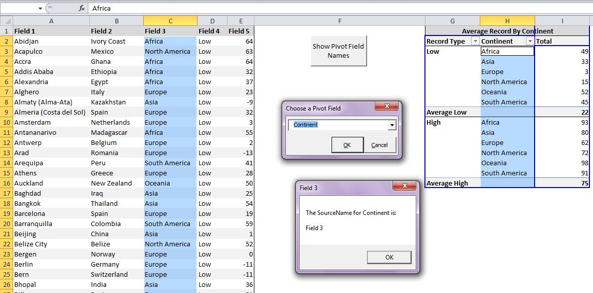
Now that we’ve got the function and the form, let’s choose something! I’ve got some code below that lists all the visible fields in a pivot table. When one is picked, the data range for the field is highlighted, along with the source column in the table, and the fields source name is displayed:

Sub ShowPivotFieldInfo()
Dim pvt As Excel.PivotTable
Dim lo As Excel.ListObject
Dim StartingCell As Excel.Range
Dim i As Long
Dim PivotFieldNames() As String
Dim pvtField As Excel.PivotField
Dim ChosenName As String

Set pvt = ActiveSheet.PivotTables("pvtRecordTemps")
Set lo = ActiveSheet.ListObjects("tblRecordTemps")
Set StartingCell = ActiveCell
With pvt
ReDim PivotFieldNames(1 To .VisibleFields.Count) As String
For i = 1 To .VisibleFields.Count
PivotFieldNames(i) = .VisibleFields(i).Name
Next i
ChosenName = GetChoiceFromChooserForm(PivotFieldNames, "Choose a Pivot Field")
If ChosenName = vbNullString Then
Exit Sub
End If
Set pvtField = .PivotFields(ChosenName)
With pvtField
Union(.DataRange, lo.ListColumns(.SourceName).DataBodyRange).Select
MsgBox Title:=.SourceName, _
Prompt:="The SourceName for " & ChosenName & " is:" & vbCrLf & vbCrLf & .SourceName
End With
StartingCell.Select
End With
End Sub

This type of code can be useful when the PivotField names have been changed drastically from their underlying SourceNames, especially if the SourceNames are cryptic, similar, and there’s lots of them. In the picture below the SourceNames in the table were “Field 1”, “Field 2”, etc., but were changed to meaningful names like “Continent” in the pivot table.

Here’s the sample workbook for your downloading pleasure.

A Prefix Function to Save You From VBA Magic Numbers, Sometimes

Posted on March 6, 2012 by Doug Glancy

Magic Numbers in Formulas

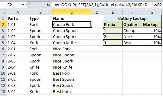
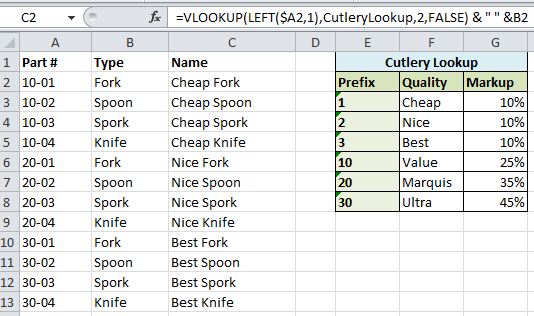
The last post referred to “magic numbers” and the pitfalls of using them in formulas. An example might be this product list, where the quality level is represented by a single digit before the dash in the part number, the “quality prefix.”

The formula generating the name in C2 is a simple one. It does a lookup of the quality prefix – 1, 2, or 3 – in the “Cutlery Lookup” table, yielding a quality of “Cheap,” “Nice” or “Best.” This is added to the product type, resulting in a name such as “Nice Spork.”

=VLOOKUP(LEFT($A2,1),CutleryLookup,2,FALSE) & " " &B2

One day the proprietors realize these lackluster brand names are a drag on sales. They create new codes and names for the products, adding a 0 to the quality prefix and new quality descriptions to the table. They then print up 2,000 parts lists, failing to notice that the formula is still generating the same lousy names.

This is due to the magic number “1” in the “VLOOKUP(LEFT($A2,1)” part. It still specifies the length of the quality prefix as 1, meaning the lookup is still seeking the prefixes 1, 2 and 3. (Admittedly, their luck was bad in choosing new codes that didn’t result in #NA and in leaving in the old ones, but they were probably forced to by other bad design practices.)

A more robust approach is to have the formula look for the dash separating the quality code from the rest of the product number, like:

=VLOOKUP(LEFT($A2,SEARCH("-",$A2)-1),CutleryLookup,2,FALSE) & " " &B2

This will accommodate different length prefixes.

Magic Numbers and Prefixes in VBA

Prefixes in VBA can also lead to magic numbers. Say you have a workbook with some worksheets identified by the prefix “final” in the name. To process these sheets you might write code like:

Dim ws As Excel.Worksheet
For Each ws In ThisWorkbook.Worksheets
If Left(ws.Name, 5) = "Final" Then
ProcessSheet ws
End If
Next ws

Of course, it’s always dangerous to use the word “final” in a name because nothing’s ever finished. So the next week when the “Really Final” worksheets need to be processed, you change your code to:

If Left(ws.Name, 5) = "Really Final" Then

and the Left function finds no sheet names whose first 5 letters are “Really Final.”

I’ve done something like this more than once, so I wrote a HasPrefix function to end it:

Function HasPrefix(StringToCheck, Prefix, Optional CaseSensitive As Boolean = False) As Boolean
If CaseSensitive Then
HasPrefix = Left((StringToCheck), Len(Prefix)) = Prefix
Else
HasPrefix = Left(LCase(StringToCheck), Len(Prefix)) = LCase(Prefix)
End If
End Function

You pass it the string to check, along with the prefix you’re checking for (and whether it’s case-sensitive if you want). It uses the length of the prefix in the Left function, so the length won’t ever be wrong.

I used this recently to check whether a workbook was located in the AppData folder in the user profile, meaning it was most likely opened from an email:

If HasPrefix(ActiveWorkbook.FullName, Environ("LOCALAPPDATA")) then

(Environ is a handy Windows function for checking on your computer’s settings and JP has an informative article on it.)

Excel Recent File Deleter

Posted on February 28, 2012 by Doug Glancy

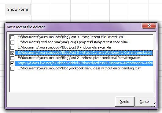
Although the downloadable file is in Excel 2003 format, I never needed one of these until Excel 2010. Now I use the recent files list a lot more, and I want to be able to tidy it up without having to right-click files one at a time. Hence the creation of this simple tool, which allows you to delete multiple entries from the list.

The form’s initialization code fills the listbox with the recent files. It sets the listbox’s style to the fabulously clunky fmListStyleOption, and MultiSelect to Extended. This means you can select multiple files using the control and shift keys. You can’t uncheck an item though, except by selecting another.

With Me.lstRecentItems
For i = 1 To Application.RecentFiles.Count
Me.lstRecentItems.AddItem Application.RecentFiles(i).Path
Next i
.ListStyle = fmListStyleOption
'you can use ctrl and shft to select multiple files
.MultiSelect = fmMultiSelectExtended
.ListIndex = -1
End With

The UserForm also has code from Andy Pope for making the form resizable, which I tinkered with a bit.

The Delete button code loops backwards through the listbox, deleting the corresponding file if the item is selected. It goes backwards for the same reason you delete rows from bottom to top – otherwise the indexing gets messed up and you delete the wrong files.

Private Sub cmdDelete_Click()
Dim i As Long

With Me.lstRecentItems
'If nothing's chosen
If .ListIndex = -1 Then
GoTo exit_point
End If
For i = .ListCount - 1 To 0 Step -1
If .Selected(i) Then
'List is zero-based, RecentFiles is a one-based collection
Application.RecentFiles(i + 1).Delete
End If
Next i
End With
'If you're looking at the Home screen this will update it
Application.ScreenUpdating = True

exit_point:
CloseForm

End Sub

I’d like it if you could bring the “pinned” items to the top of the listbox, but I don’t see any properties or objects to control that. Recentfiles seems to be simply indexed with the most recent first.

If you play around with this and, like me, delete all the files from your list, you can fill it back up with fictitious ones.

Sub FillMostRecentList()
Dim i As Long

For i = 1 To 20
Application.RecentFiles.Add ("c:/test" & i)
Next i
Application.ScreenUpdating = True
End Sub

Download the Recent File Deleter zip file.

A Workbook-Hooker with no Ribbon-related fatalities

Posted on February 24, 2012 by Doug Glancy

I’ve been working on an addin that uses application-level events to “hook” certain “target” workbooks as they open, in order to control menus and other functionality for the target workbooks. I like this setup because the code is all in the addin, so code updates don’t bother users and they don’t have to enable macros.

The Basics

The application class is created when the addin starts, and application-level events track the opening and closing of target workbooks. When a target opens, a workbook class is instantiated. That gets added to a dictionary object that contains all currently open target workbooks. The workbook class shows the ribbon tab when the workbook is activated and hides it when the workbook is deactivated.

I had never created an addin like this using ribbon menus. Creating a new ribbon group is easy using Andy Pope’s RibbonX Visual Designer. And I added the ribbon loss-of-state insurance Ron de Bruin demonstrates. But the ribbon did cause problems when I tried to address a couple of potential usage situations.

The Tricky Parts

If the addin is not checked in the Addins dialog, I want it to behave well when a user does check it. This means that if a target workbook is already open, the menu should be shown when the addin starts. The menu should also be shown if a user opens Excel by clicking on a target workbook in Windows Explorer. I tried to set this up in the addin’s ThisWorkbook module by calling initialization code from the Addin_Install and Workbook_Open events. However, this consistently crashed Excel in these two situations. Somehow my code was colliding with the ribbon’s instantiation. I tried to solve this by delaying initialization with Application.OnTime. This worked for the addin-activation scenario, but not for the Windows Explorer one. My code was somehow trying to run at the same time, or before, the ribbon’s code.

Finally, finally, it hit me that the solution was to call all my initialization code from the Ribbon_OnLoad event. That seems to have fixed the problem, and now there’s no code in the addin’s ThisWorbook module at all.

One other thing I learned was that an application-level Workbook_Open event is fired when you attempt to re-open an open workbook, either from Windows Explorer or in Excel. This could lead to trying to re-add a workbook to the Dictionary if the user accidentally tried to open an already open workbook, so I just re-load the dictionary each time.

The Code

(You can also follow the link at the end of this post to downdoad the addin and two targets.)

Here’s the Application Class module, called clsApplication. Along with hooking target workbooks when they open, it removes them from the collection when they’re closed, using the application’s BeforeClose and Deactivate events.

Public WithEvents App As Excel.Application
Private mboolWbClosing As Boolean

Private Sub App_WorkbookOpen(ByVal wb As Workbook)
If WbIsTargetWorkbook(wb) Then
FillDictionary
End If
End Sub

Private Sub App_WorkbookBeforeClose(ByVal wb As Workbook, Cancel As Boolean)
'The last close might have been cancelled
mboolWbClosing = False
If gdicTesterWorkbooks.Exists(wb.Name) Then
'It might be closing, but the close might be cancelled
mboolWbClosing = True
End If
End Sub

Private Sub App_WorkbookDeactivate(ByVal wb As Workbook)

If mboolWbClosing Then
'Okay, it's really closing
If gdicTesterWorkbooks.Exists(wb.Name) Then
gdicTesterWorkbooks.Remove wb.Name
End If
mboolWbClosing = False
End If
End Sub

This is the clsTargetWorkbook class.

Public WithEvents wb As Excel.Workbook

Private Sub Class_Initialize()
SetRibbonVisibility True
End Sub

Sub wb_Activate()
SetRibbonVisibility True
End Sub

Sub wb_Deactivate()
SetRibbonVisibility False
End Sub

Last is a module with the remaining code. It includes global variables to track the comings and goings of the ribbon, along with the class and dictionary declarations. Below that is the section that helps retrieve the ribbon reference should it be lost, followed by the subs for the actual ribbon events. Finally, there’s routines to manage the application class and dictionary, test for target workbooks, and show and hide the ribbon. (It probably goes without saying that the real version doesn’t use workbook names to test for target workbooks.)

'thanks to Rory Archibald and Ron de Bruin for Ribbon
'loss-of-state prevention code
'http://www.rondebruin.nl/ribbonstate.htm

Public gRibbon As IRibbonUI
Public cApplication As clsApplication
Public cTargetWorkbook As clsTargetWorkbook
Public gdicTesterWorkbooks As Object
Public gboolShowRibbonTab As Boolean

#If VBA7 Then
Public Declare PtrSafe Sub CopyMemory Lib "kernel32" Alias "RtlMoveMemory" (ByRef destination As Any, ByRef source As Any, ByVal length As Long)
#Else
Public Declare Sub CopyMemory Lib "kernel32" Alias "RtlMoveMemory" (ByRef destination As Any, ByRef source As Any, ByVal length As Long)
#End If

#If VBA7 Then
Function GetRibbon(ByVal lRibbonPointer As LongPtr) As Object
#Else
Function GetRibbon(ByVal lRibbonPointer As Long) As Object
#End If

Dim objRibbon As Object
CopyMemory objRibbon, lRibbonPointer, LenB(lRibbonPointer)
Set GetRibbon = objRibbon
Set objRibbon = Nothing
End Function

Public Sub Ribbon_onLoad(ribbon As IRibbonUI)
Set gRibbon = ribbon
ThisWorkbook.Names.Add Name:="RibbonPointer", RefersTo:=ObjPtr(ribbon)
ThisWorkbook.Saved = True

'only do our initialization after the ribbon's

InitializeGlobals
FillDictionary
End Sub

Sub InvalidateRibbon()
If gRibbon Is Nothing Then
Set gRibbon = GetRibbon(Replace(ThisWorkbook.Names("RibbonPointer").RefersTo, "=", ""))
End If
gRibbon.Invalidate
End Sub

Public Sub grpRibbonTester_getVisible(control As IRibbonControl, ByRef returnedVal)
returnedVal = gboolShowRibbonTab
End Sub

Public Sub cmdTester_onAction(control As IRibbonControl)
MsgBox "testing"
End Sub

Sub InitializeGlobals()
Set cApplication = New clsApplication
Set cApplication.App = Application
Set gdicTesterWorkbooks = CreateObject("Scripting.Dictionary")
End Sub

Sub FillDictionary()
Dim wb As Excel.Workbook
Dim cTargetWorkbook As clsTargetWorkbook

Set gdicTesterWorkbooks = Nothing
Set gdicTesterWorkbooks = CreateObject("Scripting.Dictionary")
For Each wb In Workbooks
If WbIsTargetWorkbook(wb) Then
Set cTargetWorkbook = New clsTargetWorkbook
Set cTargetWorkbook.wb = wb
gdicTesterWorkbooks.Add cTargetWorkbook.wb.Name, cTargetWorkbook
End If
Next wb
End Sub

Function WbIsTargetWorkbook(wb As Excel.Workbook)
If wb.Name = "Target1.xlsx" Or wb.Name = "Target2.xlsx" Then
WbIsTargetWorkbook = True
End If
End Function

Sub SetRibbonVisibility(boolRibbonVisible As Boolean)
gboolShowRibbonTab = boolRibbonVisible
InvalidateRibbon
End Sub

The Download, Should You So Desire

A zipped file with the addin, and two target workbooks. Install the addin, open the workbooks, or vice-versa.

Attach Current Workbook to Current Email

Posted on February 13, 2012 by Doug Glancy

I email workbooks all the time. Sometimes I send them unprompted in brand-new emails, in which case Excel’s “Send as Attachment” command works great. More often though, I attach them to a reply, in which case it doesn’t.

In addition, there are other traits of “Send as Attachment” which can be irksome.

It locks the workbook until you close the email. Invariably I see something I want to change and then stab pointlessly at the workbook until I notice Outlook blinking.
It doesn’t prompt you to save the workbook if you’ve made changes.
it doesn’t let you know if Outlook’s not open.

To remedy these issues I had to (yay!) write some code. Here it is:

Sub Attach_Current_Wb_To_Current_Email()

'This requires a reference to Microsoft Outlook #.# Object Library

Dim outApp As Outlook.Application
Dim OutMail As Outlook.MailItem

If ActiveWorkbook Is Nothing Then
MsgBox ("No active workbook.")
GoTo Exit_Point
End If
If ActiveWorkbook.Path = vbNullString Then
MsgBox ("This workbook has never been saved.")
GoTo Exit_Point
End If
If ActiveWorkbook.Saved = False Then
If MsgBox(prompt:="Changes have been made since last save." & vbCrLf & _
"Continue?", Buttons:=vbOKCancel + vbQuestion) = vbCancel Then
GoTo Exit_Point
End If
End If
On Error Resume Next
Set outApp = GetObject(, "Outlook.Application")
On Error GoTo 0
If outApp Is Nothing Then
If MsgBox(prompt:="Outlook isn't open." & vbCrLf & "Open and create a new email?", _
Buttons:=vbOKCancel + vbQuestion) = vbOK Then
Set outApp = CreateObject("Outlook.Application")
Set OutMail = outApp.CreateItem(olMailItem)
OutMail.Parent.Display
OutMail.Display
Else
GoTo Exit_Point
End If
End If
With outApp
If .ActiveInspector Is Nothing Then
MsgBox "There is no open item"
GoTo Exit_Point
End If
If Not TypeOf .ActiveInspector.CurrentItem Is MailItem Then
MsgBox "Type of current item isn't email"
GoTo Exit_Point
End If
Set OutMail = .ActiveInspector.CurrentItem
If OutMail.Sent Then
MsgBox "Current email was already sent."
GoTo Exit_Point
End If
OutMail.Attachments.Add ActiveWorkbook.FullName
.ActiveInspector.Display
End With

Exit_Point:
Set outApp = Nothing
End Sub

One thing it doesn’t do that Excel’s built-in command does is send a never-saved workbook, e.g., “Book1.” In addition:

If you haven’t saved all your changes it prompts you to continue or cancel.
If Outlook isn’t open it prompts you to open it and create a new email, or cancel.
If there is no open item then it exits. Ditto if the open item isn’t an email or if the email isn’t a draft.

When Outlook is opened from the code I get the little icon and message below, same as when I use Activesync. Outlook seems to work the same as ever though.

UPDATE: JP at JP Software Technologies posted a follow-up to this.

Using Worksheet CodeNames in Other Workbooks

Posted on February 10, 2012 by Doug Glancy

VBA worksheet codenames are a handy way to refer to sheets in the same workbook. Unlike regular sheet names, they can’t be changed by the user, and so is a reliable way to refer to worksheets in your code.

One thing about codenames is they’re not qualifiable. If you have a sheet codenamed “wsPivot,” you can’t refer to it as ThisWorkbbook.wsPivot. As a painfully verbose coder who declares variables as Excel.This and Office.That and can barely resist typing Application.WorksheetFunction.Max, wsPivot feels abrupt. Whose pivot is it anyways?

The fact that you’re using codenames often means you’re thinking about other users, and allowing them to rename worksheets without breaking your code. Since you’re obviously considerate, you’re probably also separating your code into an addin, so that you can maintain and improve it without disturbing users’ data. Unfortunately, because you can’t qualify codenames, you can’t code something like Workbooks(“Data.xlsx”).wsPivot. So to take advantage of the codenames in other workbooks I use this function:

Function GetWsFromCodeName(wb As Workbook, CodeName As String) As Excel.Worksheet
Dim ws As Excel.Worksheet

For Each ws In wb.Worksheets
If ws.CodeName = CodeName Then
Set GetWsFromCodeName = ws
Exit For
End If
Next ws
End Function

You can then code something like:

Dim wsPivot as Excel.Worksheet
Set wsPivot = GetWsFromCodeName(Workbooks(“Data.xlsx”), “wsPivot”)

and away you go.

goofy code

Posted on February 7, 2012 by Doug Glancy

The other day I needed to increment some footnotes for a document that gets published yearly. The footnotes look something like:

(8,11)

I needed to increment them all by three and there are a few pages, so of course I wrote some VBA. The line that prompted this post removes the left and right parentheses, then Splits the remaining string with comma as the delimiter, and assigns the resulting array to a variant. Here it is:

SplitCell = Split(Replace(Replace(cell.Value2, ")", ""), "(", ""), ",")

I admit I’m easily amused, but that is some funny looking code.

Re-Apply Pivot Table Conditional Formatting

Posted on February 4, 2012 by Doug Glancy

I often use conditional formatting in pivot tables, often to add banding to detail rows and highlights to total rows. I like conditional formatting in XL 2010 for the most part, but sometimes it’s persnickety. It seems to change its mind from day-to-day about what’s allowed.

One well-known problem is that if you apply conditional formatting to both your row fields and the data items, like this:

and then refresh it, the formatting is wiped from the data (values) area, as shown below:

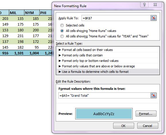
There are a couple of ways to fix this. One is to specifically apply the formats to the values area(s), a new feature as of Excel 2007. Conditional formats added this way aren’t cleared by pivot table refreshes:

This works fairly well as long as your data area only includes one values field, but if you are pivoting on multiple values fields, you’ll have to add the rule for each one. And you can’t specify row fields in this dialog, so you’ll have define the formats again for those areas. And if you alter the formats you’ll have to do it all again.

For these reasons I’d rather just apply the conditional formatting to the row headings and the values area in one fell swoop. But I don’t want to visit the condtional formatting dialog to re-expand the range each time a pivot table is refreshed.

So, I wrote the code below to expand the condtional formatting from the first row label cell into all the row label and data area cells:

Sub Extend_Pivot_CF_To_Data_Area()
Dim pvtTable As Excel.PivotTable
Dim rngTarget As Excel.Range
Dim rngSource As Excel.Range
Dim i As Long

'check for inapplicable situations
If ActiveSheet Is Nothing Then
MsgBox ("No active worksheet.")
Exit Sub
End If
On Error Resume Next
Set pvtTable = ActiveSheet.PivotTables(ActiveCell.PivotTable.Name)
If Err.Number = 1004 Then
MsgBox "The cursor needs to be in a pivot table"
Exit Sub
End If
On Error GoTo 0

With pvtTable
'format conditions will be applied to row headers and values areas
Set rngTarget = Intersect(.DataBodyRange.EntireRow, .TableRange1)
'set the format condition's source to the first cell in the row area
Set rngSource = rngTarget.Cells(1)
With rngSource.FormatConditions
For i = 1 To .Count
'reset each format condition's range to row header and values areas
.Item(i).ModifyAppliesToRange rngTarget
Next i
End With

'display isn't always refreshed otherwise
Application.ScreenUpdating = True
End With
End Sub

The key to this code is the ModifyAppliesToRange method of each FormatCondtion. This code identifies the first cell of the row label range and loops through each format condition in that cell and re-applies it to the range formed by the intersection of the row label range and the values range, i.e., the banded area in the first image above.

This method relies on all the conditional formatting you want to re-apply being in that first row labels cell. In cases where the conditional formatting might not apply to the leftmost row label, I’ve still applied it to that column, but modified the condition to check which column it’s in.

This function can be modified and called from a SheetPivotTableUpdate event, so when users or code updates a pivot table it re-applies automatically. I’ve also added this macro to the Pivot Table Context Menu and some days it gets used a lot.