yoursumbuddy

Filter and Sort a Listbox With a Helper Table

Posted on November 21, 2015 by Doug Glancy

I’ve been attempting to bend the Recent Files folder to my will for creating my own recent files form in Excel. My motivation is that Recent Files in Excel 2013 is one step further removed than in 2010. Now I’ve got a form that accesses all the Excel files in Windows Recent folder. I learned some interesting things putting it together, like how to extract a shortcut’s path in VBA. Even more interesting – instead of filtering and sorting the form’s main listbox using Like functions, arrays and collections, I just pull all the file data into a structured table and use it as the listbox’s source. When I want to sort or filter the listbox I just sort or filter the table and re-populate the listbox from the table. Much easier! No multi-dimensional array quicksorts or dictionaries required.

In actual use, the sheet with the table is hidden (it’s in my utility addin), but above is a picture of the form and the table working together.

Background

The Windows Recent Files list is some kind of semi-virtual folder that contains a bunch of shortcuts to the files you’ve opened since, well, I’m not sure when. In my Windows 10 and Windows 7 computers the path

Environ("APPDATA")\Roaming\Microsoft\Windows\Recent

gets me there.

One interesting thing about the Recent folder is that it contains workbooks that you create with code, which isn’t necessarily true in Excel’s Recent list. It also contains addins.

The folder looks like this:

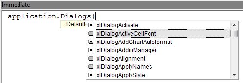
It’s chock-full of all kinds of shortcuts. At first I thought I’d just use a FileBrowserDialog with the filter set to .xls* but that doesn’t work because the file types are really all .lnk. You can enter “.xl” in the Search box in the upper right and it will filter to just Excel files, but I can’t find a way to get something into the Search box using VBA.

So next I just plunked all the filenames into a sheet and added hyperlinks to the files that still exist (just like Excel’s recent files list, the shortcuts can outlive the files):

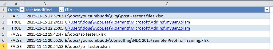
That kind of works, isn’t a great interface for something like this. The thing that really doesn’t work is that without VBA you can’t click multiple hyperlinks at once.

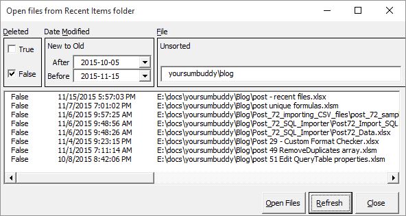
So instead I turned that table into the source for a listbox on a userform. It’s got columns showing whether the file has been deleted, its modified date and full path:

Filtering and Sorting the Listbox using the Tables Sort and Filter Objects

There it is nicely filtered to files that haven’t been deleted and other stuff sorted from newest to oldest, etc. And in order to get those nicely sorted dates, I just turned on the macro recorder and fiddled with some table-sorting VBA that it generated. Here’s the routine for the click event for the date-sorting label:

Private Sub lblFIleSort_Click()
Dim SourceTable As Excel.ListObject

If Me.lblFIleSort.Caption = "Unsorted" Then
Me.lblFIleSort.Caption = "A to Z"
ElseIf Me.lblFIleSort.Caption = "A to Z" Then
Me.lblFIleSort.Caption = "Z to A"
ElseIf Me.lblFIleSort.Caption = "Z to A" Then
Me.lblFIleSort.Caption = "A to Z"
End If
Me.lblDateSort = "Unsorted"

Set SourceTable = ThisWorkbook.Worksheets("RecentFiles").ListObjects("tblRecentFiles")
With SourceTable.Sort
.SortFields.Clear
.SortFields.Add Key:=SourceTable.ListColumns("File").Range, _
SortOn:=xlSortOnValues, _
Order:=IIf(Me.lblFIleSort.Caption = "A to Z", xlAscending, xlDescending), DataOption:=xlSortTextAsNumbers
.Header = xlYes
.Orientation = xlTopToBottom
.Apply
End With
FillLstRecentFiles
End Sub

That’s some pretty simple sorting code for a three-column listbox! The code for filtering it by filename is even shorter:

Private Sub txtFileFilter_Change()
Dim SourceTable As Excel.ListObject

Set SourceTable = ThisWorkbook.Worksheets("RecentFiles").ListObjects("tblRecentFiles")
SourceTable.Range.AutoFilter Field:=3, Criteria1:="=*" & Me.txtFileFilter.Text & "*", Operator:=xlAnd
FillLstRecentFiles
End Sub

The last line of each sub above calls the FillLstRecentFiles subroutine, which plunks the visible rows in the helper table into the listbox:

Sub FillLstRecentFiles()
Dim SourceTable As Excel.ListObject
Dim VisibleList As Excel.Range
Dim SourceTableArea As Excel.Range
Dim SourceTableRow As Excel.Range
Dim Source() As String
Dim i As Long

Me.lstRecentItems.Clear
Set SourceTable = ThisWorkbook.Worksheets("RecentFiles").ListObjects("tblRecentFiles")
On Error Resume Next
Set VisibleList = SourceTable.DataBodyRange.SpecialCells(xlCellTypeVisible)
On Error GoTo 0
If VisibleList Is Nothing Then
GoTo Exit_Point
End If
For Each SourceTableArea In VisibleList.Areas
For Each SourceTableRow In SourceTableArea.Rows
i = i + 1
ReDim Preserve Source(1 To 3, 1 To i)
Source(1, i) = SourceTableRow.Cells(1)
Source(2, i) = SourceTableRow.Cells(2)
Source(3, i) = SourceTableRow.Cells(3)
Next SourceTableRow
Next SourceTableArea
'If there's just one row
If i = 1 Then
Me.lstRecentItems.Clear
Me.lstRecentItems.AddItem (Source(1, 1))
Me.lstRecentItems.List(0, 1) = Source(2, 1)
Me.lstRecentItems.List(0, 2) = Source(3, 1)
Else
Me.lstRecentItems.List = WorksheetFunction.Transpose(Source)
End If

The main thing about the code above is that it cycles through the discontiguous Areas of the filtered table.

I’ve taken this code and added it to my main utility addin. Every time I open the utility it creates the sheet with the source table. When the form is closed the table gets deleted. It’s not terribly fast on a network when it first parses through all the files, so I don’t know how much I’ll actually use it. But I’m pretty sure I’ll be using listbox helper tables.

Have You Ever Used a Table Like This?

I’m curious whether you’ve ever used a table as a listbox helper like this. If so, how well did it work?

Download

Here’s a download so you can try it out . It also has some nifty code for getting a shortcut’s path and other treats as well.

Delete Unselected Sheets From Workbook

Posted on October 15, 2015 by Doug Glancy

My time is short and so is my code. As a sort of companion piece to the recent post on removing filters from all but the selected columns, here’s some VBA to delete unselected sheets from a workbook. It’s a type of action I find useful. Often before I send a workbook to somebody I want to delete all but one or two sheets. Sure, I could select them, right click, choose delete and answer the confirmation prompt, but I’m not a young man. My time is precious, and since deleting sheets kills the Undo stack anyways, why not do it with code?

I could use two nested loops to test whether each sheet is one of the selected sheets, but I like this better:

Sub DeleteUnselectedSheets()
Dim SelectedSheetsCount As Long

If ActiveWorkbook Is Nothing Then
MsgBox "No active workbook."
Exit Sub
End If

SelectedSheetsCount = ActiveWindow.SelectedSheets.Count
If MsgBox("Really?", vbYesNo, "Delete Unselected Sheets") = vbNo Then
Exit Sub
End If

ActiveWindow.SelectedSheets.Move before:=ActiveWorkbook.Sheets(1)
Do Until ActiveWorkbook.Sheets.Count = SelectedSheetsCount
Application.DisplayAlerts = False
ActiveWorkbook.Sheets(SelectedSheetsCount + 1).Delete
Application.DisplayAlerts = True
Loop
End Sub

You’ll notice that I chickened out and put a confirmation dialog in there. Common sense got the better of me.

The Move command keeps the SelectedSheets in the same order and moves them to the leftmost positions. At that point only the first one is selected, which is why we saved the number of selected sheets at the beginning. The Do Until loop then deletes all the sheets with a higher index than the count of originally selected sheets.

I tested it on charts and hidden sheets and it worked fine:

Selection.ListObject and Selection.PivotTable

Posted on October 4, 2015 by Doug Glancy

In recent posts about using VBA to work with filters I’ve used ActiveCell.ListObject to test whether I’m dealing with a filtered table or a filtered range. At one point it occurred that maybe I should be looking at the Selection’s ListObject instead. For various reasons that doesn’t work, but it made me wonder how Selection.ListObject gets evaluated. For example, what if it spans two tables? And, while we’re at it what about Selection.PivotTable?

To be clear, everything said about Selection in this post actually applies to the more general Range object. It’s just that Selection is the range I’m interested in.

Selection.PivotTable

Let’s start with Pivot Tables. Excel’s help actually says exactly how Range.PivotTable is handled:

Returns a PivotTable object that represents the PivotTable report containing the upper-left corner of the [Selection].

So,

Selection.PivotTable

returns an error with the selection below because its upper-left corner is outside the pivot:

But this selection will return the pivot table because the upper-left cell of the selection intersects the pivot table:

Selection.ListObject

The rules for ListObjects, or at least what I’m guessing are the rules, are different. There’s nothing I can find in Help, so here’s what I made up:

Returns the ListObject intersected by the Selection. If more than one ListObject intersects the Selection, the ListObject that was created earliest is returned.

None of the pivot table’s “upper-left corner” stuff. If the selection intersects the table, the table is returned. So below

Selection.Listobject

returns Table3.

When the Selection intersects multiple ListObjects, it looks to me like Selection.ListObject returns the one that was created earliest. With the selection below, that means that it returns Table1.

In Conclusion

Now I have even more reasons to never use Selection.ListObject or Selection.PivotTable! They’re both quirky, and I don’t think I could expect users to know that if they select more than one table, they’ll get the oldest one (or for that matter, that they’d get any one). And for a pivot table, it would be kind of fussy to insist the upper-left corner of the selection be in the pivot table.

I’m sticking with ActiveCell. I think that’s the way Range.PivotTable and Range.Selection should have been designed as well. In other words, like Range.PivotTable does, only using ActiveCell instead of the upper-left corner.

Remove Filters From Other Columns

Posted on October 1, 2015 by Doug Glancy

Here’s another in what’s turning out to be a series of posts on AutoFiltering. This time it’s a bit of code to remove filters from all the columns except those that are part of the current selection. The idea is kind of like “Close Other Tabs” in Fireox or Notepad++. It works for Tables and plain old filtered ranges. I wrote it the other day while working on a mile-wide list with various fancy filters, most of which I wanted to get rid of.

It’s not much code, and hopefully it’s self-explanatory. (If not, you know where to find me.)

Sub ClearFiltersFromOtherColumns()
Dim i As Long
Dim AutoFltr As Excel.AutoFilter

If ActiveSheet Is Nothing Then
MsgBox "No active worksheet."
Exit Sub
End If
'Determine the range with the filter depending on whether it's a Table or not
If Not ActiveCell.ListObject Is Nothing Then
Set AutoFltr = ActiveCell.ListObject.AutoFilter
Else
Set AutoFltr = ActiveCell.Parent.AutoFilter
End If
If AutoFltr Is Nothing Then
MsgBox "The selection is not within filtered table or range"
Exit Sub
End If
If Union(Selection, AutoFltr.Range).Address <> AutoFltr.Range.Address Then
MsgBox "Please make sure all cells are within the same table or filtered area."
Exit Sub
End If

For i = 1 To AutoFltr.Filters.Count
If AutoFltr.Filters(i).On And _
(Intersect(Selection.EntireColumn, AutoFltr.Range.Columns(i)) Is Nothing) Then
AutoFltr.Range.AutoFilter Field:=i
End If
Next i
End Sub

The part I like is how it narrows down to a aingle AutoFilter object regardless of whether you’re working with a ListObject or just a filtered range. I’m not sure I knew there was such an object until I read Mike Alexander’s post on A Better Way to Copy Filtered Rows Using VBA.

My Happy Birthday Contribution

Posted on September 30, 2015 by Doug Glancy

As Debra, Mike and others have mentioned today is Excel’s birthday. Woohoo!

I’ve been busy with actual paying Excel side jobs and other life stuff (which apparently is more “important” than blogging).

I did take this picture at my workplace the other day and want to share it with you. These bumper stickers are all around the building – just more proof of the awesomeness of my job. This was the first time I’d noticed this one:

So Happy Birthday Excel.

I believe in you. And trust you – even though you’re over 30.

Get Word Instance Functions

Posted on August 8, 2015 by Doug Glancy

Submitted for your approval. Three functions. Functions to do a simple job. Do it well. Or not. You be the judge.

Yes, I’m trying something new and hoping to drag you along. Don’t worry, it’s just a poll.

A poll about what?
I haven’t automated Word for quite a bit and so, to ease into it, I noodled around with all-purpose functions to find or create a Word instance.

Function Specs
This function, as I imagine it, would have one option with three choices. Or is that one choice with three options?

1. Return only an existing instance of Word. If no instances are open, return nothing.
2. Return an existing instance of Word. If none exists, create a new one.
3. Create a new instance of Word whether or not one’s already open.

That’s not what I want you to vote on. I think we can all agree there’s a time and place for each of these options.

What I want to know is which of the following functions you like best. They all do the same thing, with slightly different approaches.

Function #1 – Enums: I love ’em, or at least the idea of them. In this case we can use their bitwise ANDing capability to shorten, and perhaps obfuscate.

Public Enum WordInstanceType
ExistingInstance = 1
NewInstance = 2
End Enum

Function GetWordInstance(InstanceType As WordInstanceType) As Object
Dim wd As Object

If InstanceType And ExistingInstance Then
On Error Resume Next
Set wd = GetObject(, "Word.Application")
On Error GoTo 0
End If
'If wd is nothing now it's either because there were no existing instances
'and/or we asked for New
If (InstanceType And NewInstance) And wd Is Nothing Then
Set wd = CreateObject("Word.Application")
End If
Set GetWordInstance = wd
End Function

Function #2 – FallThrough: It’s got an ugly pattern, but it matches the way I think about it. No enum, so you’d have to look at the function to figure out what strings it recognizes. That’s pretty ugly too, so maybe you’d want to change it to an enum.

Function GetWordInstance2(InstanceType As String) As Object
Dim wd As Object

If InstanceType = "ExistingInstance" Or InstanceType = "ExistingThenNew" Then
On Error Resume Next
Set wd = GetObject(, "Word.Application")
On Error GoTo 0
'If we only want Existing, then we either got it or not
If InstanceType = "ExistingInstance" Then
Set GetWordInstance2 = wd
Exit Function
End If
End If
'If wd is nothing now it's either because
'we specified ExistingThenNew and there were no existing instances
'or we specified NewInstance
If wd Is Nothing Then
Set wd = CreateObject("Word.Application")
End If
Set GetWordInstance2 = wd
End Function

Function #3 – Plodding Boy, I’m really selling these, huh? Like #2, no enum. It doesn’t worry about duplicated code, just lays out the steps for each option. A simple function for a simple man.

Function GetWordInstance3(InstanceType As String) As Object
Dim wd As Object

If InstanceType = "ExistingInstance" Then
On Error Resume Next
Set wd = GetObject(, "Word.Application")
On Error GoTo 0
ElseIf InstanceType = "ExistingThenNew" Then
On Error Resume Next
Set wd = GetObject(, "Word.Application")
On Error GoTo 0
If wd Is Nothing Then
Set wd = CreateObject("Word.Application")
End If
ElseIf InstanceType = "NewInstance" Then
Set wd = CreateObject("Word.Application")
End If

Set GetWordInstance3 = wd
End Function

[poll id=”2″]

Dynamically Resize Form Controls With Anchors

Posted on August 1, 2015 by Doug Glancy

Every once in a while I work on a VB.Net project. The coolest was building an interface connecting an ArcGIS front-end to a SQL Server backend… but that’s another story. One thing I always enjoy about Visual Studio, besides the post-1900s IDE, is the forms. They have many fine features, like rich textboxes you’re allowed to use, data-connected listviews and, perhaps my favorite, dynamically resizable controls. The resizing behavior is set using left, right, top and bottom “anchors.” You set the anchors right in the Properties dialog box:

So of course, I decided to create anchors for my VBA forms. And I think I’ve succeeded:

My Form With Anchored Controls

The form above has two frames, a listbox, three textboxes and two commandbuttons. Their moorings are shown in this table:

How Do Anchors Work?

If you use only one anchor in a pair, like only the Left anchor, then the control moves when the form is resized, maintaining the same distance between the control and the left edge of its parent container. Its size doesn’t change. If you choose both Left and Right anchors then the control grows or shrinks horizontally to fit the parent container. It’s kind of like having left-justified, right-justified or distributed text in a cell:

In this imperfect analogy, the words are the controls and the cells are the parent containers. The same concept applies to Top and Bottom anchors.

Coding the Anchors

I used to do this kind of thing piecemeal by relating the position of one control relative to its form or another control:

It works, but it’s cumbersome and requires the use of things like a WIDTH_PADDING constant, an indication that I don’t quite know what I’m doing.

It took a while to figure out the logic for handling all the form’s controls no matter where the are on the form, what types of anchors they have and whether they’re inside another control or not. At first my formulas still looked a lot like the code above, attempting to accommodate the borders around parent controls and such.

The secret I found is to just relate the anchors to the original height and width of their parent control, whether that parent is the form itself or a frame within the form. Then you can just apply the change in width or height of the parent to the position and size of the child control:

The code to do this is in a class which you instantiate and populate from the form:

Public Sub ResizeControls()
Dim i As Long

For i = LBound(m_ControlsAnchorsAndVals) To UBound(m_ControlsAnchorsAndVals)
With m_ControlsAnchorsAndVals(i)
If .AnchorTop And .AnchorBottom Then
.ctl.Top = .StartingTop
.ctl.Height = Application.WorksheetFunction.Max(0, .StartingHeight + _
(.ctl.Parent.InsideHeight - .ParentStartingHeight))
ElseIf .AnchorTop And Not .AnchorBottom Then
.ctl.Top = .StartingTop
ElseIf Not .AnchorTop And .AnchorBottom Then
.ctl.Top = .StartingTop + (.ctl.Parent.InsideHeight - .ParentStartingHeight)
End If
If .AnchorLeft And .AnchorRight Then
.ctl.Left = .StartingLeft
.ctl.Width = Application.WorksheetFunction.Max(0, .StartingWidth + _
(.ctl.Parent.InsideWidth - .ParentStartingWidth))
ElseIf .AnchorLeft And Not .AnchorRight Then
.ctl.Left = .StartingLeft
ElseIf Not .AnchorLeft And .AnchorRight Then
.ctl.Left = .StartingLeft + (.ctl.Parent.InsideWidth - .ParentStartingWidth)
End If
End With
Next i
End Sub

m_ControlsAnchorsAndVals is an array of types, one element for each control. The type specifies which anchors apply to that control, the control’s original dimensions and its parent’s original dimensions:

Private Type ControlAnchorsAndValues
ctl As MSForms.Control
AnchorTop As Boolean
AnchorLeft As Boolean
AnchorBottom As Boolean
AnchorRight As Boolean
StartingTop As Double
StartingLeft As Double
StartingHeight As Double
StartingWidth As Double
ParentStartingHeight As Double
ParentStartingWidth As Double
End Type

Here’s the Userform code that fills the array of Types, instantiates the class and assigns the eight controls and their anchors:

Private Sub UserForm_Activate()
'We know how many controls we're dealing with
Dim ControlsAndAnchors(1 To 8) As ControlAndAnchors

'Chip Pearson code
MakeFormResizable Me, True
ShowMinimizeButton Me, False
ShowMaximizeButton Me, False

With ControlsAndAnchors(1)
Set .ctl = Me.Frame1
.AnchorTop = True
.AnchorLeft = True
.AnchorBottom = True
.AnchorRight = True
End With
With ControlsAndAnchors(2)
Set .ctl = Me.Frame2
.AnchorTop = True
.AnchorBottom = True
.AnchorRight = True
End With

'... etc

With ControlsAndAnchors(8)
Set .ctl = Me.CommandButton2
.AnchorBottom = True
.AnchorRight = True
End With

Set cFormResizing = New clsFormResizing
cFormResizing.Initialize Me, ControlsAndAnchors
End Sub

Add a little Chip Pearson form resizing code and you’re good to go.

Some Important or Perhaps Interesting Stuff to Know if You Try This

It’s important to add the controls to the array in order of their hierarchy. If you resize a control before its parent is resized it won’t work.
The WithEvents userform object seems to lack a Resize event. It does have a Layout event, which occurs whenever the form or any control on it is moved or resized. I could have worked with that, but instead I call the class’s ResizeControls subroutine from the form’s Resize event.
This project makes use of Chip Pearson’s excellent API form code, which allows you to resize, and add maximize and minimize buttons to, a form.
After finishing this I did a search and found that Andy Pope (of course!) did something like it ten years ago. He uses an enum, which is always fun, and has some different features, like setting a minimum control size. Unless I’m mistaken though, his code relates the change in control size or position only to the overall form, not to the control’s parent container. This can lead to oddness if you have two side-by-side frames containing controls.

Download

This download contains the code and form. It also has a copy of the table shown above that has the anchors listed for each control. I tied the table to the code so you can change the values of the anchors, run the form, and see how it behaves.

Be careful, or you might get something like this:

Pivot Multiple Worksheets

Posted on July 20, 2015 by Doug Glancy

As I’ve mentioned before, these days I use Excel more and more for developing and testing SQL code. As part of that I often compare of sets of output from SQL. And as part of that I sometimes I find it useful to pivot multiple worksheets.

For example, I just finished a project of translating a query from one data warehouse to another. The new database has a completely different schema than the old – new tables, new fields, new behaviors. My goal was to develop a query that returned the same results from the new database as those from the old.

To compare the outputs, I created two tables (listobjects) in a single workbook. The first table had a connection to the old data warehouse and uses the old query as its Command Text. The second table is connected to the new data warehouse, and was where I’d test the SQL I was developing.

Especially at first, there were quite a few differences in the output of these two queries in these two tables. Comparing the outputs in a pivot table let me see these differences clearly, both in summary and in detail.

Here’s a very simple example using my trusty pie data. In this example I have two different tables on two sheets with slightly different pie orders. Here’s the output from data warehouse 1…

and here it is from data warehouse 88b…

I conveniently placed differences in the Quantity column near the top, so you may be able to just pick them out by eye. And you may even have caught the one date field discrepancy. However, after combining the two tables into one, adding a “Source” column and then pivoting, the differences become easy to pick out, especially with a little conditional formatting:

In the pivot above, “2”s in the Grand Total column represent all the records where the two queries returned the same results. The “1”s point to the discrepancies.

This is a flexible and powerful comparison method. Benefits include:

You can quickly add or subtract fields from the pivot to pinpoint the differences.
You can change the orders of the fields.
If you add subtotals you can then double-click on those with disrepancies to drill down to just those results.

For a while I created these combined source tables manually, just pasting the two sets of results together, adding a column “Source” column with “DW_1” and “DW_88b.” This worked fairly well, but after several times it cried out for automation.

The VBA below keys off of selected sheets in a workbook. Just select the ones you want to pivot and then run the code. Here you can see that both sheets are selected, and I’ve added the “Pivot Multiple Sheets” macro to the tab’s right-click menu (with MenuRighter, of course).

The code first collects all the data necessary for the connection and then closes the source workbook. (I did this to avoid memory leaks or whatever it is that makes things go wonky if the workbook is open at the same time I’m creating a connection to it.) It uses that data to create the Source and SQL strings. The SQL is just a series of SELECTS, one for each selected worksheet, connected with UNION ALLs.

The newly created worbook contains a table with the connection to the source workbook and a pivot table pointed at that table. The table’s “Source” field becomes a column in the pivot table, containing the names of the two or more worksheets. The rest of the table columns become pivot table row fields. The connection in this workbook is live, so that if you make changes to the source they will appear in this workbook once you refresh the data and pivot:

Sub Pivot_Multiple_Sheets()

Dim wbToPivot As Excel.Workbook
Dim SheetsToPivot As Excel.Sheets
Dim SourceFullName As String
Dim SourceString As String
Dim wbWithPivot As Excel.Workbook
Dim wsWithQueryTable As Excel.Worksheet
Dim SheetsToPivotCount As Long
Dim SheetsToPivotNames() As String
Dim qt As Excel.QueryTable
Dim i As Long
Dim SqlSelects() As String
Dim sql As String
Dim pvt As Excel.PivotTable
Dim pvtField As Excel.PivotField

If ActiveWorkbook Is Nothing Then
MsgBox "No active workbook."
Exit Sub
End If
Set wbToPivot = ActiveWorkbook

If Not wbToPivot.Saved Then
MsgBox "Please save this workbook before running." & vbCrLf & _
"Workbook will be closed by this utility" & _
"after the process is completed."
Exit Sub
End If

'This code acts on the Selected Sheets
Set SheetsToPivot = wbToPivot.Windows(1).SelectedSheets
If SheetsToPivot.Count = 1 Then
MsgBox "Please select two or more worksheets (no charts)."
Exit Sub
End If

SheetsToPivotCount = SheetsToPivot.Count

For i = 1 To SheetsToPivotCount
If Not TypeName(SheetsToPivot(i)) = "Worksheet" Then
MsgBox "Please select two or more worksheets (no charts)."
Exit Sub
End If
Next i

SourceFullName = wbToPivot.FullName
ReDim SheetsToPivotNames(1 To SheetsToPivotCount)
For i = 1 To SheetsToPivotCount
SheetsToPivotNames(i) = SheetsToPivot(i).Name
Next i
'Change Selection to only one sheeet
SheetsToPivot(1).Select
'Close the source workbook before creating the new one and its connections
'Save it so not prompted
wbToPivot.Close True

Set wbWithPivot = Workbooks.Add
'Delete any extra worksheets
For i = wbWithPivot.Worksheets.Count To 2 Step -1
Application.DisplayAlerts = False
wbWithPivot.Worksheets(i).Delete
Application.DisplayAlerts = True
Next i
Set wsWithQueryTable = wbWithPivot.Worksheets(1)
wsWithQueryTable.Name = "Data Table"
'Don't know why this is needed, but otherwise .CommandText line below fails
wsWithQueryTable.Activate

'I got rid of a lot of fields in connection - still seems to work
SourceString = "ODBC;DSN=Excel Files;DBQ=" & SourceFullName
'Create an array of SELECT statements
ReDim SqlSelects(1 To SheetsToPivotCount)
For i = 1 To SheetsToPivotCount
SqlSelects(i) = "SELECT" & vbCrLf & _
"'" & SheetsToPivotNames(i) & "' as Source," & vbCrLf & _
"Sheet" & i & ".*" & vbCrLf & _
"FROM" & vbCrLf & _
"`" & SourceFullName & "`.[" & SheetsToPivotNames(i) & "$] AS Sheet" & i
Next i
'Connect the SELECTS with UNION ALL
For i = LBound(SqlSelects) To UBound(SqlSelects) - 1
sql = sql & SqlSelects(i) & vbCrLf & "UNION ALL" & vbCrLf
Next i
sql = sql & SqlSelects(i)

Set qt = wsWithQueryTable.ListObjects.Add(SourceType:=0, Source:=SourceString, Destination:=wsWithQueryTable.Range("$A$1")).QueryTable
With qt
.CommandText = sql
.ListObject.DisplayName = "tbl" & Format(Now(), "yyyymmddhhmmss") & Right(Format(Timer, "#0.00"), 2)
.RowNumbers = False
.FillAdjacentFormulas = False
.PreserveFormatting = True
.RefreshOnFileOpen = False
.BackgroundQuery = True
.RefreshStyle = xlInsertDeleteCells
.SavePassword = False
.SaveData = True
.RefreshPeriod = 0
.PreserveColumnInfo = True
'I like it to preserve the widths the first time it's run, and below turn it to false
.AdjustColumnWidth = True
.Refresh BackgroundQuery:=False
.AdjustColumnWidth = False
End With
wbWithPivot.Worksheets.Add
With ActiveSheet
.Name = "Pivot"
Set pvt = .Parent.PivotCaches.Create(SourceType:=xlDatabase, SourceData:=qt.ListObject.Name).CreatePivotTable(TableDestination:=.Range("A1"))
pvt.AddDataField Field:=pvt.PivotFields("Source"), Function:=xlCount
With pvt.PivotFields("Source")
.Orientation = xlColumnField
.Position = 1
End With
For Each pvtField In pvt.PivotFields
If pvtField.Name <> "Source" Then
pvtField.Orientation = xlRowField
pvtField.Position = pvt.RowFields.Count
End If
Next pvtField
End With
End Sub

To use this code put it in your Personal.xlsb or any workbook besides the one with the source data.

This code could use some more error-checking. For example, if the two sheets have a different number of columns. Even more important is the addition of whatever kind of general error handling you use so you exit gracefully from bad connection strings and other such inevitable problems.

Speaking of bad connection strings, you may notice that I’ve ditched the Default Directory, DriverId, BufferSize, MaxPageTimeOuts and whatnot from the connection. I did that to see if it worked. It did, so I never added them back. I see that they reappear in the connection properties for the table:

I ran this code in Excel 2010 and 2013. I don’t know how portable this code is to other Excel versions. I also don’t know if you’ll have performance issues if you have the source and pivot workbooks open at the same time.

If you’re interested in this topic be sure to take a look at Kirill Lapin’s method, posted on Contextures. His method keeps the source and the pivot table in one workbook, deleting the connection in between refreshes of the pivot table. I think Kirill’s method is nice for more traditional pivot table use where you want to merge different data sets with the same format, e.g., eastern and western sales regions.

I like my method because it requires no setup for the source workbook, keeps a refreshable connection and arranges the pivot table for comparison.

I’d love to hear anybody’s opinion on the stability of this method, i.e., when opening both the source and the connected data at the same time. Also, I’m curious if this code works in other versions besides 2010 and 2013. These are areas where my knowledge is pretty piecemeal, so any help would be appreciated.

Prompt to Name New Sheet

Posted on June 13, 2015 by Doug Glancy

Have you ever seen this dialog?

I’ve only seen it while running a complicated modeless form, forgetting the form was open, and then double-clicking a sheet tab to rename the sheet.

Anyways, the other day I was thinking about how often I create a new sheet and then rename it. Then I thought how cool it would be if every time I added a new sheet I was prompted to name it. Then I thought how that might actually be a pain in the butt, especially when running an addin that adds multiple sheets. So instead I wrote some code that adds a new sheet and immediately prompts for a name.

At the same time I came up with a better answer to the oft-asked question about adding a worksheet in VBA and getting a valid, unduplicated sheet name from the user.

Both of these gems require the dialog box pictured at the top of this page. Before I’d just considered it an odd reminder to close my modeless form, but now it became something I needed. My first step was to find it, which meant remembering how to show an Excel dialog from VBA and then finding the Rename Sheet one:

I searched the list looking for names starting with xlDialogRename, xlDialogSheet and xlDialogWorksheet, but no joy. I got a little nervous that my dialog wasn’t there. But searching through the whole list and trying the likely ones revealed that I was looking for xlDialogWorkbookName. It must have been a long day at the Excel factory when they named that one, but hey, close enough!

The Application.Dialogs object lets you display Excel’s built-in dialogs. It has only one method: Show. This 2003 MSDN reference is handy because it actually has a link to the arguments for each dialog type, in case you haven’t memorized them. (This information seems to be gone in Excel 2010 online and offline help):

The xlWorkbookName dialog takes two optional arguments, the name of the sheet to rename and the suggested new name. The second argument is what shows in the dialog. If you don’t specify the arguments it uses the Activesheet and its name, respectively.

You’ll notice in the screenshot above that the Show method is boolean. If the user presses OK it returns true, if they cancel it returns false. At first I thought this would be helpful in ensuring a user renames a newly-added sheet. But you really just need to add the sheet, show the dialog, and then check if it’s been renamed:

Sub PromptForNewSheetWithName()
Dim DefaultSheetName As String

ActiveWorkbook.Worksheets.Add
DefaultSheetName = ActiveSheet.Name
Application.Dialogs(xlDialogWorkbookName).Show
If ActiveSheet.Name = DefaultSheetName Then
MsgBox "You didn't name the new sheet." & vbCrLf & _
"Processing cancelled", vbExclamation
Application.DisplayAlerts = False
ActiveSheet.Delete
Application.DisplayAlerts = True
End If
End Sub

The answers I see on the web for how to prompt a user to name a new sheet all use an InputBox and involve a fair amount of validation for name length, duplicate names and illegal characters (and completely ignore the single quote issue). Using this dialog, you can let Excel do all that validation:

As for my original idea, I now have a two-line subroutine that adds a sheet and displays the dialog. I use an OnKey command in my personal macro workbook to set it to a Ctrl-Shift-F11 shortcut.

Think of the time I’ll save!

Filter Column by External List

Posted on May 13, 2015 by Doug Glancy

In a comment to my last post Jeff suggested it would be easy to modify that routine to filter a column by an external table, similar to some code he’s written for pivot tables. That would be very useful as part of a model or report, making it easy for users to update by just plopping new values into the table every week or what-have-you.

However, these days I mostly use Excel as a SQL development environment, running the SQL right in a table and then filtering and pivoting the results to figure out if my queries are working. For that reason, I really just wanted a form with a textbox where I could drop a bunch of values and filter by them. That utility, combined with the built-in filtering tools and the code from my last post would give me a lot of ways to parse my data.

And now, thanks to the wonder that is VBA, I have that utility. What’s more, so do you!

Above is the form in all its simple glory. I’d show an “After” picture, but I trust your imagination can supply that.

The UserForm VBA

Here’s the code for the main routine. It looks a lot like that in my last post, so be sure to check that out if you haven’t already:

Sub FilterList()
Dim FilterValues() As String
Dim ColNumberInFilterRange As Long
Dim FilterRange As Excel.Range
Dim InTable As Boolean
Dim CollUniqueValues As Collection
Dim i As Long

If ActiveSheet Is Nothing Then
MsgBox "No active worksheet."
Exit Sub
End If
If Me.txtValues.Text = "" Then
MsgBox "Enter at least one value to filter by"
Exit Sub
End If
With Selection
If .Cells.Count = 1 And IsEmpty(ActiveCell) Then
MsgBox "Please select a cell within one or more cells with data."
Exit Sub
End If
If Union(ActiveCell.EntireColumn, .EntireColumn).Address <> ActiveCell.EntireColumn.Address Then
MsgBox "Only select from one column"
Exit Sub
End If
'Set the range to be filtered depending on whether it's a Table or not
If Not ActiveCell.ListObject Is Nothing Then
Set FilterRange = ActiveCell.ListObject.Range
InTable = True
Else
Set FilterRange = ActiveCell.CurrentRegion
End If
If Union(Selection, FilterRange).Address <> FilterRange.Address Then
MsgBox "Please make sure all cells are within the same table or contiguous area."
Exit Sub
End If
'If not in a table and we're filtering a different area than currently filtered
'then turn the existing AutoFilter off, so no error when the new area gets filtered.
If Not InTable And ActiveSheet.AutoFilterMode Then
If ActiveSheet.AutoFilter.Range.Address <> .CurrentRegion.Address Then
ActiveSheet.AutoFilterMode = False
End If
End If

FilterValues = Split(Me.txtValues.Text, vbCrLf)
'Try to add every selected value to a collection - only unique values will succeed
Set CollUniqueValues = New Collection
For i = LBound(FilterValues) To UBound(FilterValues)
On Error Resume Next
CollUniqueValues.Add FilterValues(i)
On Error GoTo 0
Next i
'Transfer the collection to an array for the AutoFilter function
ReDim FilterValues(1 To CollUniqueValues.Count)
For i = LBound(FilterValues) To UBound(FilterValues)
FilterValues(i) = CollUniqueValues(i)
Next i
'Determine the index of the column to be filtered within the FilterRange
ColNumberInFilterRange = (.Column - FilterRange.Columns(1).Column) + 1
FilterRange.AutoFilter Field:=ColNumberInFilterRange, Criteria1:=FilterValues, Operator:=xlFilterValues
End With
End Sub

There’s one issue with this code that I haven’t solved yet. When I paste into the textbox it always puts a line feed after the last item. Unless I backspace up to the end of the last item the filter also includes blank cells, not what I’d usually want. On the other hand I don’t think I just want to get rid of that last line feed in my code because I might actually want to include a null value/blank in the filter.

Download

This download has the resizable (thanks to Chip Pearson) form for you to play with.

Next Time

Filter Using Common Household Objects!