VBA Archives - Page 3 of 8

Get Word Instance Functions

Posted on August 8, 2015 by Doug Glancy

Submitted for your approval. Three functions. Functions to do a simple job. Do it well. Or not. You be the judge.

Yes, I’m trying something new and hoping to drag you along. Don’t worry, it’s just a poll.

A poll about what?
I haven’t automated Word for quite a bit and so, to ease into it, I noodled around with all-purpose functions to find or create a Word instance.

Function Specs
This function, as I imagine it, would have one option with three choices. Or is that one choice with three options?

1. Return only an existing instance of Word. If no instances are open, return nothing.
2. Return an existing instance of Word. If none exists, create a new one.
3. Create a new instance of Word whether or not one’s already open.

That’s not what I want you to vote on. I think we can all agree there’s a time and place for each of these options.

What I want to know is which of the following functions you like best. They all do the same thing, with slightly different approaches.

Function #1 – Enums: I love ’em, or at least the idea of them. In this case we can use their bitwise ANDing capability to shorten, and perhaps obfuscate.

Public Enum WordInstanceType
ExistingInstance = 1
NewInstance = 2
End Enum

Function GetWordInstance(InstanceType As WordInstanceType) As Object
Dim wd As Object

If InstanceType And ExistingInstance Then
On Error Resume Next
Set wd = GetObject(, "Word.Application")
On Error GoTo 0
End If
'If wd is nothing now it's either because there were no existing instances
'and/or we asked for New
If (InstanceType And NewInstance) And wd Is Nothing Then
Set wd = CreateObject("Word.Application")
End If
Set GetWordInstance = wd
End Function

Function #2 – FallThrough: It’s got an ugly pattern, but it matches the way I think about it. No enum, so you’d have to look at the function to figure out what strings it recognizes. That’s pretty ugly too, so maybe you’d want to change it to an enum.

Function GetWordInstance2(InstanceType As String) As Object
Dim wd As Object

If InstanceType = "ExistingInstance" Or InstanceType = "ExistingThenNew" Then
On Error Resume Next
Set wd = GetObject(, "Word.Application")
On Error GoTo 0
'If we only want Existing, then we either got it or not
If InstanceType = "ExistingInstance" Then
Set GetWordInstance2 = wd
Exit Function
End If
End If
'If wd is nothing now it's either because
'we specified ExistingThenNew and there were no existing instances
'or we specified NewInstance
If wd Is Nothing Then
Set wd = CreateObject("Word.Application")
End If
Set GetWordInstance2 = wd
End Function

Function #3 – Plodding Boy, I’m really selling these, huh? Like #2, no enum. It doesn’t worry about duplicated code, just lays out the steps for each option. A simple function for a simple man.

Function GetWordInstance3(InstanceType As String) As Object
Dim wd As Object

If InstanceType = "ExistingInstance" Then
On Error Resume Next
Set wd = GetObject(, "Word.Application")
On Error GoTo 0
ElseIf InstanceType = "ExistingThenNew" Then
On Error Resume Next
Set wd = GetObject(, "Word.Application")
On Error GoTo 0
If wd Is Nothing Then
Set wd = CreateObject("Word.Application")
End If
ElseIf InstanceType = "NewInstance" Then
Set wd = CreateObject("Word.Application")
End If

Set GetWordInstance3 = wd
End Function

[poll id=”2″]

Dynamically Resize Form Controls With Anchors

Posted on August 1, 2015 by Doug Glancy

Every once in a while I work on a VB.Net project. The coolest was building an interface connecting an ArcGIS front-end to a SQL Server backend… but that’s another story. One thing I always enjoy about Visual Studio, besides the post-1900s IDE, is the forms. They have many fine features, like rich textboxes you’re allowed to use, data-connected listviews and, perhaps my favorite, dynamically resizable controls. The resizing behavior is set using left, right, top and bottom “anchors.” You set the anchors right in the Properties dialog box:

So of course, I decided to create anchors for my VBA forms. And I think I’ve succeeded:

My Form With Anchored Controls

The form above has two frames, a listbox, three textboxes and two commandbuttons. Their moorings are shown in this table:

How Do Anchors Work?

If you use only one anchor in a pair, like only the Left anchor, then the control moves when the form is resized, maintaining the same distance between the control and the left edge of its parent container. Its size doesn’t change. If you choose both Left and Right anchors then the control grows or shrinks horizontally to fit the parent container. It’s kind of like having left-justified, right-justified or distributed text in a cell:

In this imperfect analogy, the words are the controls and the cells are the parent containers. The same concept applies to Top and Bottom anchors.

Coding the Anchors

I used to do this kind of thing piecemeal by relating the position of one control relative to its form or another control:

It works, but it’s cumbersome and requires the use of things like a WIDTH_PADDING constant, an indication that I don’t quite know what I’m doing.

It took a while to figure out the logic for handling all the form’s controls no matter where the are on the form, what types of anchors they have and whether they’re inside another control or not. At first my formulas still looked a lot like the code above, attempting to accommodate the borders around parent controls and such.

The secret I found is to just relate the anchors to the original height and width of their parent control, whether that parent is the form itself or a frame within the form. Then you can just apply the change in width or height of the parent to the position and size of the child control:

The code to do this is in a class which you instantiate and populate from the form:

Public Sub ResizeControls()
Dim i As Long

For i = LBound(m_ControlsAnchorsAndVals) To UBound(m_ControlsAnchorsAndVals)
With m_ControlsAnchorsAndVals(i)
If .AnchorTop And .AnchorBottom Then
.ctl.Top = .StartingTop
.ctl.Height = Application.WorksheetFunction.Max(0, .StartingHeight + _
(.ctl.Parent.InsideHeight - .ParentStartingHeight))
ElseIf .AnchorTop And Not .AnchorBottom Then
.ctl.Top = .StartingTop
ElseIf Not .AnchorTop And .AnchorBottom Then
.ctl.Top = .StartingTop + (.ctl.Parent.InsideHeight - .ParentStartingHeight)
End If
If .AnchorLeft And .AnchorRight Then
.ctl.Left = .StartingLeft
.ctl.Width = Application.WorksheetFunction.Max(0, .StartingWidth + _
(.ctl.Parent.InsideWidth - .ParentStartingWidth))
ElseIf .AnchorLeft And Not .AnchorRight Then
.ctl.Left = .StartingLeft
ElseIf Not .AnchorLeft And .AnchorRight Then
.ctl.Left = .StartingLeft + (.ctl.Parent.InsideWidth - .ParentStartingWidth)
End If
End With
Next i
End Sub

m_ControlsAnchorsAndVals is an array of types, one element for each control. The type specifies which anchors apply to that control, the control’s original dimensions and its parent’s original dimensions:

Private Type ControlAnchorsAndValues
ctl As MSForms.Control
AnchorTop As Boolean
AnchorLeft As Boolean
AnchorBottom As Boolean
AnchorRight As Boolean
StartingTop As Double
StartingLeft As Double
StartingHeight As Double
StartingWidth As Double
ParentStartingHeight As Double
ParentStartingWidth As Double
End Type

Here’s the Userform code that fills the array of Types, instantiates the class and assigns the eight controls and their anchors:

Private Sub UserForm_Activate()
'We know how many controls we're dealing with
Dim ControlsAndAnchors(1 To 8) As ControlAndAnchors

'Chip Pearson code
MakeFormResizable Me, True
ShowMinimizeButton Me, False
ShowMaximizeButton Me, False

With ControlsAndAnchors(1)
Set .ctl = Me.Frame1
.AnchorTop = True
.AnchorLeft = True
.AnchorBottom = True
.AnchorRight = True
End With
With ControlsAndAnchors(2)
Set .ctl = Me.Frame2
.AnchorTop = True
.AnchorBottom = True
.AnchorRight = True
End With

'... etc

With ControlsAndAnchors(8)
Set .ctl = Me.CommandButton2
.AnchorBottom = True
.AnchorRight = True
End With

Set cFormResizing = New clsFormResizing
cFormResizing.Initialize Me, ControlsAndAnchors
End Sub

Add a little Chip Pearson form resizing code and you’re good to go.

Some Important or Perhaps Interesting Stuff to Know if You Try This

It’s important to add the controls to the array in order of their hierarchy. If you resize a control before its parent is resized it won’t work.
The WithEvents userform object seems to lack a Resize event. It does have a Layout event, which occurs whenever the form or any control on it is moved or resized. I could have worked with that, but instead I call the class’s ResizeControls subroutine from the form’s Resize event.
This project makes use of Chip Pearson’s excellent API form code, which allows you to resize, and add maximize and minimize buttons to, a form.
After finishing this I did a search and found that Andy Pope (of course!) did something like it ten years ago. He uses an enum, which is always fun, and has some different features, like setting a minimum control size. Unless I’m mistaken though, his code relates the change in control size or position only to the overall form, not to the control’s parent container. This can lead to oddness if you have two side-by-side frames containing controls.

Download

This download contains the code and form. It also has a copy of the table shown above that has the anchors listed for each control. I tied the table to the code so you can change the values of the anchors, run the form, and see how it behaves.

Be careful, or you might get something like this:

Pivot Multiple Worksheets

Posted on July 20, 2015 by Doug Glancy

As I’ve mentioned before, these days I use Excel more and more for developing and testing SQL code. As part of that I often compare of sets of output from SQL. And as part of that I sometimes I find it useful to pivot multiple worksheets.

For example, I just finished a project of translating a query from one data warehouse to another. The new database has a completely different schema than the old – new tables, new fields, new behaviors. My goal was to develop a query that returned the same results from the new database as those from the old.

To compare the outputs, I created two tables (listobjects) in a single workbook. The first table had a connection to the old data warehouse and uses the old query as its Command Text. The second table is connected to the new data warehouse, and was where I’d test the SQL I was developing.

Especially at first, there were quite a few differences in the output of these two queries in these two tables. Comparing the outputs in a pivot table let me see these differences clearly, both in summary and in detail.

Here’s a very simple example using my trusty pie data. In this example I have two different tables on two sheets with slightly different pie orders. Here’s the output from data warehouse 1…

and here it is from data warehouse 88b…

I conveniently placed differences in the Quantity column near the top, so you may be able to just pick them out by eye. And you may even have caught the one date field discrepancy. However, after combining the two tables into one, adding a “Source” column and then pivoting, the differences become easy to pick out, especially with a little conditional formatting:

In the pivot above, “2”s in the Grand Total column represent all the records where the two queries returned the same results. The “1”s point to the discrepancies.

This is a flexible and powerful comparison method. Benefits include:

You can quickly add or subtract fields from the pivot to pinpoint the differences.
You can change the orders of the fields.
If you add subtotals you can then double-click on those with disrepancies to drill down to just those results.

For a while I created these combined source tables manually, just pasting the two sets of results together, adding a column “Source” column with “DW_1” and “DW_88b.” This worked fairly well, but after several times it cried out for automation.

The VBA below keys off of selected sheets in a workbook. Just select the ones you want to pivot and then run the code. Here you can see that both sheets are selected, and I’ve added the “Pivot Multiple Sheets” macro to the tab’s right-click menu (with MenuRighter, of course).

The code first collects all the data necessary for the connection and then closes the source workbook. (I did this to avoid memory leaks or whatever it is that makes things go wonky if the workbook is open at the same time I’m creating a connection to it.) It uses that data to create the Source and SQL strings. The SQL is just a series of SELECTS, one for each selected worksheet, connected with UNION ALLs.

The newly created worbook contains a table with the connection to the source workbook and a pivot table pointed at that table. The table’s “Source” field becomes a column in the pivot table, containing the names of the two or more worksheets. The rest of the table columns become pivot table row fields. The connection in this workbook is live, so that if you make changes to the source they will appear in this workbook once you refresh the data and pivot:

Sub Pivot_Multiple_Sheets()

Dim wbToPivot As Excel.Workbook
Dim SheetsToPivot As Excel.Sheets
Dim SourceFullName As String
Dim SourceString As String
Dim wbWithPivot As Excel.Workbook
Dim wsWithQueryTable As Excel.Worksheet
Dim SheetsToPivotCount As Long
Dim SheetsToPivotNames() As String
Dim qt As Excel.QueryTable
Dim i As Long
Dim SqlSelects() As String
Dim sql As String
Dim pvt As Excel.PivotTable
Dim pvtField As Excel.PivotField

If ActiveWorkbook Is Nothing Then
MsgBox "No active workbook."
Exit Sub
End If
Set wbToPivot = ActiveWorkbook

If Not wbToPivot.Saved Then
MsgBox "Please save this workbook before running." & vbCrLf & _
"Workbook will be closed by this utility" & _
"after the process is completed."
Exit Sub
End If

'This code acts on the Selected Sheets
Set SheetsToPivot = wbToPivot.Windows(1).SelectedSheets
If SheetsToPivot.Count = 1 Then
MsgBox "Please select two or more worksheets (no charts)."
Exit Sub
End If

SheetsToPivotCount = SheetsToPivot.Count

For i = 1 To SheetsToPivotCount
If Not TypeName(SheetsToPivot(i)) = "Worksheet" Then
MsgBox "Please select two or more worksheets (no charts)."
Exit Sub
End If
Next i

SourceFullName = wbToPivot.FullName
ReDim SheetsToPivotNames(1 To SheetsToPivotCount)
For i = 1 To SheetsToPivotCount
SheetsToPivotNames(i) = SheetsToPivot(i).Name
Next i
'Change Selection to only one sheeet
SheetsToPivot(1).Select
'Close the source workbook before creating the new one and its connections
'Save it so not prompted
wbToPivot.Close True

Set wbWithPivot = Workbooks.Add
'Delete any extra worksheets
For i = wbWithPivot.Worksheets.Count To 2 Step -1
Application.DisplayAlerts = False
wbWithPivot.Worksheets(i).Delete
Application.DisplayAlerts = True
Next i
Set wsWithQueryTable = wbWithPivot.Worksheets(1)
wsWithQueryTable.Name = "Data Table"
'Don't know why this is needed, but otherwise .CommandText line below fails
wsWithQueryTable.Activate

'I got rid of a lot of fields in connection - still seems to work
SourceString = "ODBC;DSN=Excel Files;DBQ=" & SourceFullName
'Create an array of SELECT statements
ReDim SqlSelects(1 To SheetsToPivotCount)
For i = 1 To SheetsToPivotCount
SqlSelects(i) = "SELECT" & vbCrLf & _
"'" & SheetsToPivotNames(i) & "' as Source," & vbCrLf & _
"Sheet" & i & ".*" & vbCrLf & _
"FROM" & vbCrLf & _
"`" & SourceFullName & "`.[" & SheetsToPivotNames(i) & "$] AS Sheet" & i
Next i
'Connect the SELECTS with UNION ALL
For i = LBound(SqlSelects) To UBound(SqlSelects) - 1
sql = sql & SqlSelects(i) & vbCrLf & "UNION ALL" & vbCrLf
Next i
sql = sql & SqlSelects(i)

Set qt = wsWithQueryTable.ListObjects.Add(SourceType:=0, Source:=SourceString, Destination:=wsWithQueryTable.Range("$A$1")).QueryTable
With qt
.CommandText = sql
.ListObject.DisplayName = "tbl" & Format(Now(), "yyyymmddhhmmss") & Right(Format(Timer, "#0.00"), 2)
.RowNumbers = False
.FillAdjacentFormulas = False
.PreserveFormatting = True
.RefreshOnFileOpen = False
.BackgroundQuery = True
.RefreshStyle = xlInsertDeleteCells
.SavePassword = False
.SaveData = True
.RefreshPeriod = 0
.PreserveColumnInfo = True
'I like it to preserve the widths the first time it's run, and below turn it to false
.AdjustColumnWidth = True
.Refresh BackgroundQuery:=False
.AdjustColumnWidth = False
End With
wbWithPivot.Worksheets.Add
With ActiveSheet
.Name = "Pivot"
Set pvt = .Parent.PivotCaches.Create(SourceType:=xlDatabase, SourceData:=qt.ListObject.Name).CreatePivotTable(TableDestination:=.Range("A1"))
pvt.AddDataField Field:=pvt.PivotFields("Source"), Function:=xlCount
With pvt.PivotFields("Source")
.Orientation = xlColumnField
.Position = 1
End With
For Each pvtField In pvt.PivotFields
If pvtField.Name <> "Source" Then
pvtField.Orientation = xlRowField
pvtField.Position = pvt.RowFields.Count
End If
Next pvtField
End With
End Sub

To use this code put it in your Personal.xlsb or any workbook besides the one with the source data.

This code could use some more error-checking. For example, if the two sheets have a different number of columns. Even more important is the addition of whatever kind of general error handling you use so you exit gracefully from bad connection strings and other such inevitable problems.

Speaking of bad connection strings, you may notice that I’ve ditched the Default Directory, DriverId, BufferSize, MaxPageTimeOuts and whatnot from the connection. I did that to see if it worked. It did, so I never added them back. I see that they reappear in the connection properties for the table:

I ran this code in Excel 2010 and 2013. I don’t know how portable this code is to other Excel versions. I also don’t know if you’ll have performance issues if you have the source and pivot workbooks open at the same time.

If you’re interested in this topic be sure to take a look at Kirill Lapin’s method, posted on Contextures. His method keeps the source and the pivot table in one workbook, deleting the connection in between refreshes of the pivot table. I think Kirill’s method is nice for more traditional pivot table use where you want to merge different data sets with the same format, e.g., eastern and western sales regions.

I like my method because it requires no setup for the source workbook, keeps a refreshable connection and arranges the pivot table for comparison.

I’d love to hear anybody’s opinion on the stability of this method, i.e., when opening both the source and the connected data at the same time. Also, I’m curious if this code works in other versions besides 2010 and 2013. These are areas where my knowledge is pretty piecemeal, so any help would be appreciated.

Prompt to Name New Sheet

Posted on June 13, 2015 by Doug Glancy

Have you ever seen this dialog?

I’ve only seen it while running a complicated modeless form, forgetting the form was open, and then double-clicking a sheet tab to rename the sheet.

Anyways, the other day I was thinking about how often I create a new sheet and then rename it. Then I thought how cool it would be if every time I added a new sheet I was prompted to name it. Then I thought how that might actually be a pain in the butt, especially when running an addin that adds multiple sheets. So instead I wrote some code that adds a new sheet and immediately prompts for a name.

At the same time I came up with a better answer to the oft-asked question about adding a worksheet in VBA and getting a valid, unduplicated sheet name from the user.

Both of these gems require the dialog box pictured at the top of this page. Before I’d just considered it an odd reminder to close my modeless form, but now it became something I needed. My first step was to find it, which meant remembering how to show an Excel dialog from VBA and then finding the Rename Sheet one:

I searched the list looking for names starting with xlDialogRename, xlDialogSheet and xlDialogWorksheet, but no joy. I got a little nervous that my dialog wasn’t there. But searching through the whole list and trying the likely ones revealed that I was looking for xlDialogWorkbookName. It must have been a long day at the Excel factory when they named that one, but hey, close enough!

The Application.Dialogs object lets you display Excel’s built-in dialogs. It has only one method: Show. This 2003 MSDN reference is handy because it actually has a link to the arguments for each dialog type, in case you haven’t memorized them. (This information seems to be gone in Excel 2010 online and offline help):

The xlWorkbookName dialog takes two optional arguments, the name of the sheet to rename and the suggested new name. The second argument is what shows in the dialog. If you don’t specify the arguments it uses the Activesheet and its name, respectively.

You’ll notice in the screenshot above that the Show method is boolean. If the user presses OK it returns true, if they cancel it returns false. At first I thought this would be helpful in ensuring a user renames a newly-added sheet. But you really just need to add the sheet, show the dialog, and then check if it’s been renamed:

Sub PromptForNewSheetWithName()
Dim DefaultSheetName As String

ActiveWorkbook.Worksheets.Add
DefaultSheetName = ActiveSheet.Name
Application.Dialogs(xlDialogWorkbookName).Show
If ActiveSheet.Name = DefaultSheetName Then
MsgBox "You didn't name the new sheet." & vbCrLf & _
"Processing cancelled", vbExclamation
Application.DisplayAlerts = False
ActiveSheet.Delete
Application.DisplayAlerts = True
End If
End Sub

The answers I see on the web for how to prompt a user to name a new sheet all use an InputBox and involve a fair amount of validation for name length, duplicate names and illegal characters (and completely ignore the single quote issue). Using this dialog, you can let Excel do all that validation:

As for my original idea, I now have a two-line subroutine that adds a sheet and displays the dialog. I use an OnKey command in my personal macro workbook to set it to a Ctrl-Shift-F11 shortcut.

Think of the time I’ll save!

Filter Column by External List

Posted on May 13, 2015 by Doug Glancy

In a comment to my last post Jeff suggested it would be easy to modify that routine to filter a column by an external table, similar to some code he’s written for pivot tables. That would be very useful as part of a model or report, making it easy for users to update by just plopping new values into the table every week or what-have-you.

However, these days I mostly use Excel as a SQL development environment, running the SQL right in a table and then filtering and pivoting the results to figure out if my queries are working. For that reason, I really just wanted a form with a textbox where I could drop a bunch of values and filter by them. That utility, combined with the built-in filtering tools and the code from my last post would give me a lot of ways to parse my data.

And now, thanks to the wonder that is VBA, I have that utility. What’s more, so do you!

Above is the form in all its simple glory. I’d show an “After” picture, but I trust your imagination can supply that.

The UserForm VBA

Here’s the code for the main routine. It looks a lot like that in my last post, so be sure to check that out if you haven’t already:

Sub FilterList()
Dim FilterValues() As String
Dim ColNumberInFilterRange As Long
Dim FilterRange As Excel.Range
Dim InTable As Boolean
Dim CollUniqueValues As Collection
Dim i As Long

If ActiveSheet Is Nothing Then
MsgBox "No active worksheet."
Exit Sub
End If
If Me.txtValues.Text = "" Then
MsgBox "Enter at least one value to filter by"
Exit Sub
End If
With Selection
If .Cells.Count = 1 And IsEmpty(ActiveCell) Then
MsgBox "Please select a cell within one or more cells with data."
Exit Sub
End If
If Union(ActiveCell.EntireColumn, .EntireColumn).Address <> ActiveCell.EntireColumn.Address Then
MsgBox "Only select from one column"
Exit Sub
End If
'Set the range to be filtered depending on whether it's a Table or not
If Not ActiveCell.ListObject Is Nothing Then
Set FilterRange = ActiveCell.ListObject.Range
InTable = True
Else
Set FilterRange = ActiveCell.CurrentRegion
End If
If Union(Selection, FilterRange).Address <> FilterRange.Address Then
MsgBox "Please make sure all cells are within the same table or contiguous area."
Exit Sub
End If
'If not in a table and we're filtering a different area than currently filtered
'then turn the existing AutoFilter off, so no error when the new area gets filtered.
If Not InTable And ActiveSheet.AutoFilterMode Then
If ActiveSheet.AutoFilter.Range.Address <> .CurrentRegion.Address Then
ActiveSheet.AutoFilterMode = False
End If
End If

FilterValues = Split(Me.txtValues.Text, vbCrLf)
'Try to add every selected value to a collection - only unique values will succeed
Set CollUniqueValues = New Collection
For i = LBound(FilterValues) To UBound(FilterValues)
On Error Resume Next
CollUniqueValues.Add FilterValues(i)
On Error GoTo 0
Next i
'Transfer the collection to an array for the AutoFilter function
ReDim FilterValues(1 To CollUniqueValues.Count)
For i = LBound(FilterValues) To UBound(FilterValues)
FilterValues(i) = CollUniqueValues(i)
Next i
'Determine the index of the column to be filtered within the FilterRange
ColNumberInFilterRange = (.Column - FilterRange.Columns(1).Column) + 1
FilterRange.AutoFilter Field:=ColNumberInFilterRange, Criteria1:=FilterValues, Operator:=xlFilterValues
End With
End Sub

There’s one issue with this code that I haven’t solved yet. When I paste into the textbox it always puts a line feed after the last item. Unless I backspace up to the end of the last item the filter also includes blank cells, not what I’d usually want. On the other hand I don’t think I just want to get rid of that last line feed in my code because I might actually want to include a null value/blank in the filter.

Download

This download has the resizable (thanks to Chip Pearson) form for you to play with.

Next Time

Filter Using Common Household Objects!

Filter Column By All Selected Values

Posted on May 3, 2015 by Doug Glancy

Excel’s Filter by Selected Cell’s Value is a popular command, and for good reason. It’s a quick way to filter the data that you’re looking at. There are times when I’d like to take it one step further and filter by the values of multiple cells. So I wrote some code and added a “Filter By All Selected Values” item to my right-click menu. It works just like Filter by Selected Cells except you can select multiple cells.

Here’s the result:

There’s one situation where this feature is especially handy: that’s when I need to see all instances in one column of items that match a single characteristic in another column. For instance, “I want to see all the pie orders from customers who have ordered Red Velvet Cheesecake.”

I could do this operation with a Countif formula like…

=COUNTIFS([Name],[@Name],[Pie],"Red velvet cheesecake")>0

and then filter to all the rows that return TRUE.

But this new routine allows me to do this without helper columns.

Here’s How

First, select “Red Velvet Cheesecake,” then right-click and choose the regular old Filter > Filter by Selected Cell’s Value. You’ll see all the rows with that value.

Next, select all the customers and run the “Filter by All Selected Values” code. This will filter the Customers column by only the three currently visible names. This is the part that I don’t see how to do easily without this code.

Finally, clear the filter from “Pies” that you set in the first step. The result will match that above with the COUNTIFS formula.

A Brief Commercial Announcement

If you’re wondering how I got those things in my context menu see the MenuRighter page.

The Code

The code I wrote works for tables and contiguous areas.

Sub Filter_By_All_Selected_Values()

Dim FilterValues() As String
Dim i As Long, j As Long
Dim ColNumberInFilterRange As Long
Dim FilterRange As Excel.Range
Dim InTable As Boolean
Dim CollUniqueValues As Collection
Const MAX_FILTER_CELLS As Long = 10000

'Make sure we don't select cells hidden by filter
With Selection.SpecialCells(xlCellTypeVisible)
If Union(ActiveCell.EntireColumn, .EntireColumn).Address <> ActiveCell.EntireColumn.Address Then
MsgBox "Only select from one column"
Exit Sub
End If
If .Areas.Count = 1 And .Rows.Count = 1 Then
MsgBox "Select more than one cell"
Exit Sub
End If
If .Cells.Count > MAX_FILTER_CELLS Then
MsgBox "Cannot select more than " & MAX_FILTER_CELLS & " cells."
Exit Sub
End If

'Set the range to be filtered depending on whether it's a Table or not
If Not ActiveCell.ListObject Is Nothing Then
Set FilterRange = ActiveCell.ListObject.Range
InTable = True
Else
Set FilterRange = ActiveCell.CurrentRegion
End If
If Union(Selection, FilterRange).Address <> FilterRange.Address Then
MsgBox "Please make sure all cells are within the same table or contiguous area."
Exit Sub
End If

'If not in a table and we're filtering a different area than currently filtered
'then turn the existing AutoFilter off, so no error when the new area gets filtered.
If Not InTable And ActiveSheet.AutoFilterMode Then
If ActiveSheet.AutoFilter.Range.Address <> .CurrentRegion.Address Then
ActiveSheet.AutoFilterMode = False
End If
End If

'Try to add every selected value to a collection - only unique values will succeed
Set CollUniqueValues = New Collection
For i = 1 To .Areas.Count
For j = 1 To .Areas(i).Cells.Count
On Error Resume Next
CollUniqueValues.Add .Areas(i).Cells(j).Text, .Areas(i).Cells(j).Text
On Error GoTo 0
Next j
Next i
'Transfer the collection to an array for the AutoFilter function
ReDim Preserve FilterValues(1 To CollUniqueValues.Count)
For i = LBound(FilterValues) To UBound(FilterValues)
FilterValues(i) = CollUniqueValues(i)
Next i
'Determine the index of the column to be filtered within the FilterRange
ColNumberInFilterRange = (.Column - FilterRange.Columns(1).Column) + 1
FilterRange.AutoFilter Field:=ColNumberInFilterRange, Criteria1:=FilterValues, Operator:=xlFilterValues
End With
End Sub

How it Works

The first part of the code consists of a few checks to make sure the selection is more than one cell, is only in one column, and that you haven’t selected a huge number of cells. This last one is controlled by the MAX_FILTER_CELLS constant. I set it at 10,000, a number that ran with no noticeable delay.

After that the code checks whether the ActiveCell is in a table or not. In either case, it assigns the range to be filtered to the FilterRange variable. It then checks that all the currently selected cells reside within either the same table or contiguous area.

The code uses our old friend the “get unique items using a collection” trick. It then applies a filter to the FilterRange.

The trickiest part of the code was defining the conditions that require an Exit Sub, such as selecting in multiple columns. That’s mainly because something like “Selection.Columns.Count” only returns the count of columns in the first Area of a selection. The same thing applies to the Selection’s CurrentRegion. I got around these limitations by using Union and the fact that Selection.Address returns the address for all areas in the the selection.

Download

Here’s a workbook with the code and the pie orders table so you can easily try the filtering I did above.

Missing Addin User Warning

Posted on April 23, 2015 by Doug Glancy

I develop workbooks that require an addin for some of their functionality. For example, a set of school staffing models whose addin allows for selecting data sources, building pivot tables and saving timestamped copies. I like this structure because it’s very maintainable – it’s much easier to fix a bug or add a feature in one addin than it is to try to track down a bunch of workbooks and update their VBA. Easier on me and better for my users. Of course, people’s computers get re-imaged or replaced and IT departments are unlikely, to say the least, to re-install a VBA addin. Folks often don’t realize their addins are gone and that’s why their model is broken. Yesterday I got an idea about how to warn users about a missing addin. I’m still tinkering with it, but the idea is quite simple.

Use a UDF in the Addin

What I did was create the world’s simplest UDF and put it in the addin:

Public Function IsAddinLoaded() As Boolean
IsAddinLoaded = True
End Function

It doesn’t have to be boolean. It could be a string and return “Cult of the Flying Spaghetti.” That’s because it’s only purpose is to fail when it’s not there.

Missing Addin = Missing UDF = opportunity for IsError formula. So, for example, in cell A1 of the addin-dependent workbook put something like:

="Ye Olde Spreadsheet " & IF(ISERROR(isaddinloaded()*TODAY()),"requires the Green Eyeshade Addin!
Please install it.","is Good to Go")

Then add a little conditional formatting based on the missing addin condition and you get something like this. (I tried referring to the UDF directly in the conditional formatting, but it looks like that’s not allowed.)

The formula contains a volatile function: TODAY. That’s so if the addin is uninstalled the error is activated with the next change to the worksheet. I’d like to avoid the volatile function and I’ve tried to do this in the VBA itself, but haven’t figured out anything yet.

The message does change to the non-warning one as soon as the addin is installed.

The addin a very simple one made up just for this post. It’s called Green Eyeshade and it’s for modernizing old spreadsheets like this one. Its ribbon tab is shown when a workbook meeting certain criteria is opened. Here’s the ribbon tab:

And here’s the modernization button in action (wonderful what you can find by googling “Peltier pie charts”).

This idea could also be applied to the problem of warning users to enable VBA when opening xlsm files. I’ve never been a big fan of the “hide everything in the workbook except a warning page” although I do like Mike Alexander’s clear explanation. Anyways, something like this might work as an alternative in that case too.

Download

Here’s a zip file with the xlam addin and the target “olde spreadsheet” xlsx file.

Tweaking View Side by Side

Posted on March 15, 2015 by Doug Glancy

I use View Side by Side a lot. That means I spend a bit of time fiddling with the two windows because I don’t always want each to take up half the space. I often make one smaller and then adjust the second to have it fill the rest of the screen. This weekend I set about tweaking View Side by Side to adjust one window when the other is resized.

Along the way I learned a few interesting things. The most important to this code was figuring out how tell if View Side by Side is activated. I also noticed some issues with View Side by Side in Excel 2013.

Below is a screenshot of what happens when you resize a window in View Side by Side. You can see that it needs to be followed up with some more fiddling to snug the lower window up against the upper one:

The code I came up with is in an application-level event. It uses a function to test whether View Side by Side is active. It’s designed to work in Excel 2010 (and 2007, although untested) as well as 2013. The 2013 tweaks were a little trickier, because Application.Height returned the same thing as Window.Height in 2013. This means the code needs to store the lower windows top location before resizing it.

You’ll also note that I used On Error Resume Next more freely than normally. After all we’re just resizing windows here, and it’s easier than testing for odd things like heights less than zero:

Public WithEvents app As Excel.Application

'application-level event in a class module
Private Sub app_WindowResize(ByVal Wb As Workbook, ByVal Wn As Window)
Dim UpperWindow As Excel.Window
Dim LowerWindow As Excel.Window
Dim OldLowerWindowTop As Double
Dim LowerWindowChange As Double

'See function below
If SideBySideOn Then
With Application
.EnableEvents = False
'assign the two windows,
'based on which is uppermost
If .Windows(1).Top <= .Windows(2).Top Then
Set UpperWindow = .Windows(1)
Set LowerWindow = .Windows(2)
Else
Set UpperWindow = .Windows(2)
Set LowerWindow = .Windows(1)
End If

'easy way to deal with heights less than zero, etc.
On Error Resume Next
'for Excel 2010 could just use Application.Height
'but in Excel 2013 each window is its own Application
If ActiveWindow.Caption = UpperWindow.Caption Then
OldLowerWindowTop = LowerWindow.Top
LowerWindow.Top = UpperWindow.Top + UpperWindow.Height
LowerWindowChange = LowerWindow.Top - OldLowerWindowTop
LowerWindow.Width = UpperWindow.Width
LowerWindow.Height = LowerWindow.Height - LowerWindowChange
Else
UpperWindow.Height = LowerWindow.Top
UpperWindow.Width = LowerWindow.Width
End If
On Error GoTo 0
.EnableEvents = True
End With
End If
End Sub

This code only responds to resizes involving the two horizontal borders in the middle, as well as the right-hand borders. So, if you drag the top border of the upper window nothing adjusts.

Application-Level Event

The sample workbook sets an application-level class in its Workbook_Open event. I’ve posted on this before and there’s lots of good info out there, like this Chip Pearson page.

How Do You Tell if View Side by Side is Active?

That’s an interesting question! Here’s what I tried:

First, I looked for some type of setting, like Application.ViewSideBySideEnabled. I can’t find one. Instead there’s two methods: CompareSideBySideWith and the rather drastic-sounding BreakSideBySide.
It would be nice if you could just get the state of the Ribbon’s View Side by Side button. That would tell you whether it’s active or not. But I don’t know of any way to do this.
You can, however, check the state of Excel 2003-style command buttons. So I tried looking at
Application.CommandBars(1).Controls("Window").Controls("Compare Side By Side With").State

to check whether it’s pressed. It turns out that control – ID 7698 – has no state. Instead it switches captions from “Compare Side by Side With” (followed by a workbook name if there’s only one choice) to “Close Side By Side.”
Based on #3 I considered getting the state by checking whether the first five letters are “Close” or “Compa.” But of course that wouldn’t work for folks with non-English Excel versions, and I generally shy away from using labels when I can use ID’s.
So, finally I decided to use the state of the “Reset Window Position” button. This button is only enabled when View Side by Side is active.

This leads to a one-line function that checks that button’s status using its ID of 7874. There is one final wrinkle, which is that this button doesn’t appear by default in the Excel 2003 “Window” toolbar. By default it lives only in the “Add Command” toolbar which was the one that appeared in 2003 when you modified a toolbar. No problem. We can find number 7874 wherever it lives by searching through all the commandbars using FindControl. Here’s the function:

Function SideBySideOn() As Boolean
'Reset Window Position
SideBySideOn = CommandBars.FindControl(ID:=7874).Enabled
End Function

Here’s how it looks with the code running:

Other Stuff Learned Along the Way

If you click the Reset Window Position button with the lower window selected, it moves to the top. I’d never noticed that.
There is no Window.Move event
View Side by Side in Excel 2013 is harder to use. This makes sense, since one of the biggest changes in Excel 2013 is the change to a Single-Document-Interface, making it easier to separate workbooks to multiple monitors. However it’s hard to grab the right edge of a workbook inside View Side by Side. And, as noted above, Application.Height and Window.Height now seem to be the same thing. This makes sense most of the time, but not when you are in View Side by Side mode and trying to compare the height of one of the workbooks/windows to the overall height.

Download!

Here you are my friend.

Autofilter VBA Operator Parameters

Posted on February 22, 2015 by Doug Glancy

The other day I was flipping back and forth between two tables with related sets of data and comparing the rows for one person in each set. I do this kind of thing all the time and often end up filtering each table to the same person, location, date, or whatever, in order to compare their rows more easily. I thought “Wouldn’t it be great to write a little utility that filters a field in one table based on the same criteria as a filter in another table?” Like many questions that begin with “Wouldn’t it be great to write a little utility” this one led me on a voyage of discovery. The utility isn’t finished, but I know a lot more about Autofilter VBA operator parameters.

My biggest discovery is that the parameters used in the Range.Autofilter method to set a filter don’t always match the properties of the Filter object used to read the criteria. For instance, you filter on a cell’s color by passing its RGB value to Criteria1. But when reading the RGB value of a Filter object, Criteria1 suddenly has a Color property. More about this and some other such wrinkles as we go along.

I also realized there are a bunch of xlDynamicFilter settings – like averages and dates – that all use the same operator and are specified by setting the Criteria1 argument.

I also noticed a typo in the xlFilterAllDatesInPeriodFebruray operator. I wonder if anybody has ever even used it?

The Basics – Setting a Filter in VBA

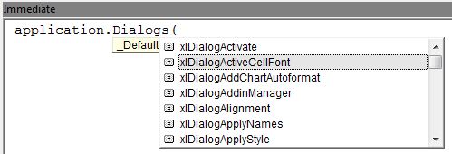
To review the basics of setting Autofilters in VBA you can peruse the skimpy help page. To add a bit to that, let’s return to one of my favorite tables:

Its columns have several characteristices on which you can filter, including text, dates and colors. Here it’s filtered to names that contain “A”, pies with the word “Berry”, dates in the current month and puke-green:

To filter the pies to just berry you have to load their names into an array and set Criteria1 and Operator like:

Sub PieTableFilters()
Dim lo As Excel.ListObject
Dim BerryPies As Variant

Set lo = ActiveWorkbook.Worksheets("pie orders").ListObjects(1)
BerryPies = Array("Strawberry", "Blueberry", "Razzleberry", "Boysenberry")
lo.DataBodyRange.AutoFilter field:=2, _
Criteria1:=BerryPies, Operator:=xlFilterValues
End Sub

Discovery #1 – An xlFilterValues Array Set With Two Values Becomes an xlOR Operator:
To read the filter created by the code above, I’d still use the xlFilterValues operator and read the array from Criteria1. However, if the column was filtered to only two types of pies, I’d use the xlOR operator and Criteria1 and Criteria2. This is unchanged since Johh Walkenbach posted about Stephen Bullen’s function to read filters settings for Excel 2003.

Similarly, if I set a filter with a one-element array, e.g., only one type of pie, and then read the filter operator it returns a 0.

The Basics, Continued – Setting a Color Filter

Here’s how to set the filter for the last column. It’s based on cell color. Note that it works for Conditional Formatting colors as well as regular fill colors:

lo.DataBodyRange.AutoFilter field:=4, _
Criteria1:=8643294, Operator:=xlFilterCellColor

Here 8643294 is the RGB value of that greenish color. In order to determine that RGB in code, you need to use something like:

Set lo = ActiveWorkbook.Worksheets("pie orders").ListObjects(1)
Debug.Print lo.AutoFilter.Filters(4).Criteria1.Color

Discovery #2 – The Filter.Criteria1 Property Sometimes has Sub-Properties, Like Color:
Note that the RGB isn’t in Criteria1 – it’s in Criteria1.Color, a property I only discovered by digging around in the Locals window:

Also note that there are a bunch of other properties there, like Pattern, etc.

Further, if a column is filtered by conditional formatting icon (yes you can do that) using the xlFilterIcon(10) parameter then Criteria1 contains an Icon property. This property is numbered 1 to 4 (I think) and relates to the position of the icon in its group.

Discovery #3: xlDynamicFilter and Its Many Settings
The xlFilterDynamic operator, enum 11, is a broad category of settings. You narrow them down in Criteria1. So, for instance, you can filter a column to the current month like:

lo.DataBodyRange.AutoFilter field:=3, _
Criteria1:=XlDynamicFilterCriteria.xlFilterThisMonth, _
Operator:=xlFilterDynamic

This is a good time to mention the chart below that contains all of these xlDynamicFilter operators and their enums. Looking at it you’ll note that in addition to a whole lot of date filters (all of which appear in Excel’s front end as well) there’s also the Above Average and Below Average filters.

Discovery #4: Top 10 Settings Are Weird

To set a Top 10 item in VBA you do something like this:

lo.DataBodyRange.AutoFilter field:=4, _
Criteria1:=3, Operator:=xlTop10Items

Here, I’ve actually filtered column 4 to the top three items (As stated in Help, Criteria1 contains the actual number of items to filter). If I look at the filter settings for that column in the table I’ll see that Number Filters is checked and the dialog shows “Top 10.” That makes sense.

However if we look at the locals window right after the line above is executed, we see that the number 3 which we coded in Criteria1 is replaced by a greater than formula:

Further, if I then wanted to apply this filter to another column based only on what I’m able to read in VBA, I’d have to change it to:

'ValuePulledFromAnotherFilter contains ">=230"
lo.DataBodyRange.AutoFilter field:=4, _
Criteria1:=ValuePulledFromAnotherFilter

Note that I don’t use an operator at all. We could also use xlFilterValues or xlOr. Using nothing best reflects what shows in the locals window, where the operator changes to 0 after the code above is executed.

The Chart

Below is a chart, contained in a OneDrive usable and downloadable workbook, that summarizes much of the above. It includes all the possible Autofilter VBA Operator parameters, as well as all the sub-parameters for the xlFilterDynamic operator.

Discovery #5: February is the Hardest Month (to spell)

I like to automate things as much as possible, so generating the list of xlFilterDynamic properties was kind of a pain. To get the list of constants from the Object Browser I had to copy and paste one by one into Excel, where I cobbled together a line of VBA for each one, like:

Debug.Print “xlFilterAboveAverage: ” & xlFilterAboveAverage

Of course I saw I didn’t need to paste all the month operators into Excel since I could just drag “January” down eleven more cells and append the generated month names. Minutes saved!

But when I ran the code it choked on February. It was then I noticed that its constant is misspelled.

Two More Tips

1. Use Enum Numbers, not Constants: This misspelling of February points out a good practice when using any set of enums: use the number, not the constants. For example, use 8, not xlFilterValues. This helps in case the constants are changed in future Excel versions, and with international compatibility, late binding and, at least in this case, spelling errors. Of course it’s not nearly as readable and you have to figure out the enums.

2. The Locals Window is Your Friend: I don’t use the Locals window very much, but in working with these Autofilter settings, it was hugely helpful. It revealed things that I don’t think I’d have figured out any other way.

Conclusion – Building a Utility

Armed with my newfound knowledge, I could come close to building a utility that copies filters from one table to another, or one like the Walkenbach/Bullen filter lister linked at the beginning of this post. In most cases I could just transfer the filter by using the source Operator and Criteria1 (and Criteria2 where applicable)

But as we’ve seen, there’s a couple of filter types where the operator and/or criteria change. The worst of these is a Top 10 filter. My first thought was to count the number of unfiltered cells, but if the column has duplicates, e.g., your top value appears three times, that won’t always be accurate. In addition, other columns could be filtered which could also throw off the count.

Transferring a color scale filter would be even trickier as it’s very possible the same color wouldn’t exist in the second table.

Whew! Long post! Leave a comment if you got this far and let me know what you think.

Book1.Saved = True

Posted on January 20, 2015 by Doug Glancy

You may be familiar with VBA’s Workbook.Saved property. It’s read/write and lets you determine, or set, whether a workbook has been saved. Reading is straightforward but setting is more interesting. Declaring

MyBook.Saved = True

doesn’t actually save the workbook, it just tells Excel to act like it’s saved. So, if you don’t make any changes to the workbook and you go to close it, you won’t be prompted to save.

If you had asked me if it’s possible to set the Saved property on a never-been-saved workbook I would have said, “I don’t know, let me try it and get back to you.” Well you didn’t ask, but I’m getting back to you anyways. It turns out you can. You can open up a brand-new workbook, type “Movin’ to Montana soon” in A1 and “Gonna be a dental floss tycoon” in A2, then enter

Book1.Saved

in the immediate window, and you won’t be prompted to save if you close it.

I didn’t expect that. It kind of makes sense that you can declare an existing workbook to be saved, but one that doesn’t even have a location yet? That doesn’t sit right with the left side of my brain, which would prefer that the property be re-named to something like

Workbook.YouWontBePromptedToSaveUnlessYouChangeSomething

To expand on the above paragraph, a never-been-saved workbook doesn’t have a path. You can test the ActiveWorkbook with

ActiveWorkbook.Path = ""

, which returns True if the workbook has never been saved. I’d thought maybe setting Saved to True would change the Path property to the never-been-saved workbook location, but it doesn’t. Also, if you do decide to save, the Save As menu pops up, just as you’d hope. So it looks like setting Saved to True changes nothing except that you won’t be prompted to save.

I’ve found this useful for a certain kind of utility: one that prints out information which I want to examine but not keep. For instance, there’s a routine I use a lot that compares the sheets in two workbooks. It opens a new workbook and prints information about all the sheets in each book and whether they occur in the other book and, if so, the extent to which they match. The new workbook with the comparison is called “wbComparison,” so the last line of code is:

wbComparison.Saved = True

I know it’s a small thing, but it pleases me to look over the comparison and close it without being prompted to save.

Here’s a very simple sample for your testing pleasure:

Sub ShowZappaLyrics()
Dim wbZappa As Excel.Workbook

Set wbZappa = Workbooks.Add
With wbZappa
With .Worksheets(1)
.Cells(1, 1) = "Movin' to Montana soon"
.Cells(2, 1) = "Gonna be a Dental Floss tycoon"
End With
.Saved = True
End With
End Sub