Pivot Table Pivot Chart Navigator

This post is about navigating between pivot tables and pivot charts. The sample workbook contains a Pivot Table and Pivot Chart Navigator userform that lists the workbook’s pivot tables and takes you to them or their associated charts. The workbook also adds buttons to the chart and pivot table right-click menus. These buttons take you to the associated pivot chart or table. I used Ribbon XML for this last part since later versions of Excel don’t allow modification of the chart context menus with VBA. The downloadable workbook can be easily converted to an addin.

pivot chart context menu

I used to eschew pivot charts as far too clunky. Recently though I was given a project that contained many pivot charts. It seemed that, unless I’d just gotten much less picky (not likely), pivot charts work much better than I remembered. This impression was confirmed in a Jon Peltier post, so I know it’s true.

Using XML to Add to Right-Click Menus

As mentioned above, I’ve added a “Go to Source Pivot” button at the bottom of the chart context menu. I’d never used Ribbon XML to make a right-click menu before. The XML part is straightforward.

To create the button I used the Custom UI Editor and added a ContextMenu section to the XML. I also used the Microsoft’s NameX addin to figure out the name that refers to the chart context menu (ContextMenuChartArea) The XML for the chart and pivot table context menus is below. All of this, including links to the Custom UI Editor and the NameX addin, is covered very nicely in this MSDN post.

Since I’m already forced to use XML to modify the chart context menu, I used it for the pivot table context menu too, even though it can still be modified with VBA:

<contextMenus>
    <contextMenu idMso="ContextMenuChartArea">
     <button id="cmdGoToSourcePivot" label="Go To Source Pivot"
        onAction="cmdGoToSourcePivot_onAction"
        getVisible = "cmdGoToSourcePivot_GetVisible"/>
    </contextMenu>
    <contextMenu idMso="ContextMenuPivotTable">
     <button id="cmdGoToPivotChart" label="Go To Pivot Chart"
        onAction="cmdGoToPivotChart_onAction" />
    </contextMenu>
</contextMenus>

VBA to Go To Source Pivot
The code to go to the source pivot is similar to that in my Finding a Pivot Chart’s Pivot Table post. It looks at the charts PivotLayout property, which only exists if a chart is based on a pivot table. I use this same property in the RibbonInvalidate method to only show the “Go To Pivot Table” button when the chart is a pivot chart. That’s one thing I like about programming the ribbon: the code to show or hide tabs, buttons and other controls is generally simpler than it is when using VBA.

VBA to Go To Pivot Chart
The code to go to a pivot table’s chart loops through all chart sheets and charts on worksheets looking for one whose source range is the pivot table’s range:

Function GetPivotChart(pvt As Excel.PivotTable) As Excel.Chart
Dim wbWithPivots As Excel.Workbook
Dim ws As Excel.Worksheet
Dim chtObject As Excel.ChartObject
Dim cht As Excel.Chart

Set wbWithPivots = pvt.Parent.Parent
For Each cht In wbWithPivots.Charts
    If Not cht.PivotLayout Is Nothing Then
        If cht.PivotLayout.PivotTable.TableRange1.Address(external:=True) = pvt.TableRange1.Address(external:=True) Then
            Set GetPivotChart = cht
            Exit Function
        End If
    End If
Next cht
For Each ws In wbWithPivots.Worksheets
    For Each chtObject In ws.ChartObjects
        Set cht = chtObject.Chart
        If Not cht.PivotLayout Is Nothing Then
            If cht.PivotLayout.PivotTable.TableRange1.Address(external:=True) = pvt.TableRange1.Address(external:=True) Then
                Set GetPivotChart = cht
                Exit Function
            End If
        End If
    Next chtObject
Next ws
End Function

PivotNavigator Form
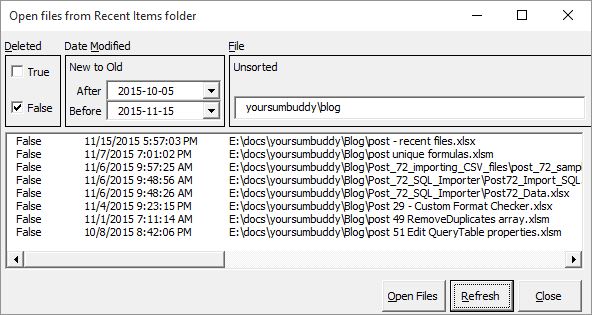
The other element of the sample workbook is a simple-yet-powerful form that navigates through a workbook’s pivot tables and pivot charts.

pivot navigator form

The form opens up with a list of all the pivot tables in the active workbook. Selecting an item in the form list takes you to the selected pivot. Use the Ctrl key with the left and right arrows to toggle between a pivot and its associated chart.

The form is modeless and responds to selection changes in the workbook, updating the list selection when you click into a different pivot or chart. This functionality uses VBA from my last post, which raises an event every time any chart in a workbook is selected.

Download
The sample workbook has the modified right-click menus, the navigation form and a button in the Developer tab to start the form. There’s even instructions!

Track ActiveCell Movement Within Selection

I searched the internet a bit before deciding that neither Excel or the forums have a way to track Activecell movement in a Selection. So, even though I don’t have the most pressing need for such an event, I spent several quality hours coding one.

The Issue
Here’s what I’m talking about. You can capture cell activation using Selection_Change code:

Private Sub Worksheet_SelectionChange(ByVal Target As Range)
Me.Range("A2") = ActiveCell.Address
Me.Range("B2") = ActiveCell.Value
End Sub

Selection Change

But this doesn’t capture cell activation within a selection, the kind that happens when you select an area and then tab through it:

No ActiveCell Change

I noticed this while creating a little ActiveCell Viewer form. My solution is to capture TAB key presses using Application.OnKey. This is a little clunky in a couple of ways, but it seems to work.

My Solution
So my userform uses OnKey to capture the Tab press when a Selection has more than one cell. Now I know when the active cell is changing within a selection, so that’s good. The hard part is that, since I’ve killed the normal Tab behavior, I have to recreate it in VBA with code that moves the ActiveCell one cell forward. Before I can do that I need to define the active cell’s location in terms of the selection.

Basically, the code cycles through each cell in each Area of the Selection. The Areas cycle through in the order they were selected. Tab cycles through each cell of an Area from top to bottom, right to left no matter how you selected the Area.

A Little More About Areas
I do believe that areas are always rectangular. If you make a selection with the control key down, each down-drag-up of the mouse represents an area. I’ve delved into this area (hah) before in the SelectTracker post. As indicated there, if you hold down Ctrl and click a cell five times you get a Selection with five Areas. Interestingly, Excel 2016 gives the unsuspecting user a bit of a hint that this is happening by making the cell a little darker with each click:

darkening Selection

Back to the Coding Process

At first, as so often happens, the VBA seemed fairly simple:

  1. Find the ActiveCell’s position within the overall Selection by looping through its Areas and through each Area’s cells.
  2. Figure out what the next (or previous) cell would be, accounting for moving from one Area to the next and hopping to the beginning of the next Area or looping back to the beginning of the whole Selection.

Then I started thinking about Selections with multiple Areas that intersect the ActiveCell. To deal with this I did two things needed to make the tabbing flow smoothly through overlapping Areas.:

  1. Created a global variable to track which of these areas was selected by the last Tab press.
  2. Created a short routine to figure out the “most recent” Area that intersects the ActiveCell

The Code
Here’s the code that identifies the Activecell’s position within the Selection’s Areas and Cells:

Private Sub SelectNextCellInSelection()

'This sub is called when the Tab key is pressed.
'The point is to be able to capture Tab key presses
'that occur within a Selection, thereby capturing movement of the Activecell.
Dim SelectionCellIndex As Long
Dim SelectionCell As Excel.Range
Dim SelectionArea As Excel.Range

For Each SelectionArea In Selection.Areas
    SelectionCellIndex = 0
    'Mod lets us cycle to the Area after we reach the last one
    SelectionAreaIndex = (SelectionAreaIndex Mod Selection.Areas.Count) + 1
    For Each SelectionCell In Selection.Areas(SelectionAreaIndex).Cells
        SelectionCellIndex = SelectionCellIndex + 1
        If SelectionCell.Address = ActiveCell.Address Then
            GoTo SelectNext
        End If
    Next SelectionCell
Next SelectionArea

SelectNext:
'Cycle to the next cell. If we're in the last one, we'll cycle to first.
SelectionCellIndex = (SelectionCellIndex Mod Selection.Areas(SelectionAreaIndex).Cells.Count) + 1
'If we're in the first cell must have gone to the next Area.
If SelectionCellIndex = 1 Then
    SelectionAreaIndex = (SelectionAreaIndex Mod Selection.Areas.Count) + 1
End If

Selection.Areas(SelectionAreaIndex).Cells(SelectionCellIndex).Activate
'Because it will get incremented next time round
SelectionAreaIndex = SelectionAreaIndex - 1
End Sub

The code above uses the Mod function to cycle back to the beginning of the next Area or of the entire Selection.

The code to cycle backwards was surpisingly more difficult. Mod didn’t work in reverse, For/Next doesn’t work in reverse, and the beginning number is the last number of the previous Area changes (not 1). So although the logic was the same, the coding was much trickier.

Putting this in a UserForm had the additional complication that the procedures assigned to a key using OnKey have to reside in a regular module. So my code has two very short routines that poke a property in the UserForm, effectively passing the action back into the form as soon as possible.

I also learned VBA’s AppActivate command which shifts the focus from the form to Excel proper. I do that at the end of the forms Activate procedure, since it’s a Viewer after all and doesn’t need the focus.

The ActiveCell Viewer
You may be wondering why you even need an ActiveCell viewer. Well, you probably don’t. But if you did, it might be to see what’s in cells with big blobs of text, or ones that are in hidden columns or rows. And its ability to view cell contents using different format strings might also be nice:

Viewer in Action

Download
Download the sample workbook and try it yourself!

Editing Shape Points for No Good Reason

Over at Bacon Bits, Mike Alexander has a nice post out yesterday on editing shape points to create custom graphics. It shows how to use a shape’s Edit Points command to create interesting dashboard icons. I haven’t used Edit Points for years, but his post inspired me to fool around with them. I ended up with a bit of code for Editing Shape Points for No Good Reason.

In Mike’s post he shows how you can edit points to modify a half-circle into a more interesting shape. His edit of a half-circle looks something like this (only better):

semicircle to wavy

I thought that was pretty cool, so then I dragged the top below the bottom:

semicircle to wavy

That was fun. Now how about some facial reconstruction for Smiley?

smiley to pointy

At this point of course I had to learn how to program these edits in VBA. The result is code that randomly messes with the edit points, along with colors:

Pointless Point Editing Code

Sub EditPointMadness()
Dim shp As Shape
Dim shpNodes As ShapeNodes
Dim CenterX As Long
Dim CenterY As Long
Dim CurrXValue As Long
Dim CurrYValue As Long
Dim ws As Excel.Worksheet
Dim pointsArray As Variant
Const PointOffset As Long = 200

Set ws = ActiveSheet
If ws.Shapes.Count = 0 Then
    ws.Shapes.AddShape msoShapeSmileyFace, 300, 300, PointOffset, PointOffset
    Exit Sub
End If
Set shp = ws.Shapes(1)
CenterX = shp.Left + (shp.Width / 2)
CenterY = shp.Top + (shp.Height / 2)
Set shpNodes = shp.Nodes
With shpNodes
    .Insert WorksheetFunction.RandBetween(1, .Count), msoSegmentCurve, msoEditingAuto, _
        WorksheetFunction.RandBetween(CenterX - PointOffset, CenterX + PointOffset), _
        WorksheetFunction.RandBetween(CenterY - PointOffset, CenterY + PointOffset), _
        WorksheetFunction.RandBetween(CenterX - PointOffset, CenterX + PointOffset), _
        WorksheetFunction.RandBetween(CenterY - PointOffset, CenterY + PointOffset), _
        WorksheetFunction.RandBetween(CenterX - PointOffset, CenterX + PointOffset), _
        WorksheetFunction.RandBetween(CenterY - PointOffset, CenterY + PointOffset)
    If Timer Mod 2 = 0 Then
        pointsArray = .Item(WorksheetFunction.RandBetween(1, .Count)).Points
        CurrXValue = pointsArray(1, 1)
        CurrYValue = pointsArray(1, 2)
        .SetPosition WorksheetFunction.RandBetween(1, .Count), _
            CurrXValue + WorksheetFunction.RandBetween(-PointOffset, PointOffset), _
            CurrYValue + WorksheetFunction.RandBetween(-PointOffset, PointOffset)
        shp.Fill.ForeColor.RGB = WorksheetFunction.RandBetween(1, 10000000)
        shp.Line.ForeColor.RGB = WorksheetFunction.RandBetween(1, 10000000)
    End If
    If Timer Mod 5 = 0 Then
        .Delete WorksheetFunction.RandBetween(1, .Count)
    End If
End With
End Sub

Every time you run the code above it adds, deletes and/or modifies another point. After a couple of times you get what I like to call “Picasso Smiley”:

smiley picasso

A few more and Smiley is getting blown into the next dimension:

smiley in the next dimension

Hopefully the code above is pretty straightforward. It leaves a few of the settings unrandomized, chiefly whether the new node is straight, shaped or a corner.

One question. How to refresh Excel between shape format changes?
One version of this code had a loop that edited the points every half second. But try as I might I couldn’t get the screen to update and show those changes. The changes would only appear after the code was finished, making a loop pointless. If anybody knows how to do this, please let us know (thereby adding some useful content to this post).

Download
Here’s a workbook with the the code and a couple of buttons to run it.

smiley edit points

Getting Pivot Table Value Field Characteristics

This post is about a bit of code that answered somebody’s Stack Overflow question, was fun to write, and taught me a few more things about the pivot table object model, which is my favorite object model. So neat, so tidy, so logical – just like pivot tables themselves.

What, you ask, do I mean by Value Field Characteristics? I mean the page, row and column fields and items that the value field is summing, counting or otherwise valuing. So in the picture below the selected value field has three row items: one each for Continent, Country and State.

value field

The Code

Here’s the code to print that same information to the Immediate window. Like the Excel tooltip in the picture it also lists the Value field name, e.g., Sum of Population, and its source field, e.g., Population. (This can be handy when you’ve modified the value field name to something like else, like “Residents.”):

Sub GetValueFieldStuff()
Dim pvtCell As Excel.PivotCell
Dim pvtTable As Excel.PivotTable
Dim pvtField As Excel.PivotField
Dim pvtItem As Excel.PivotItem
Dim pvtParentField As Excel.PivotField
Dim i As Long

On Error Resume Next
Set pvtCell = ActiveCell.PivotCell
If Err.Number <> 0 Then
    MsgBox "The cursor needs to be in a pivot table"
    Exit Sub
End If
On Error GoTo 0

If pvtCell.PivotCellType <> xlPivotCellValue Then
    MsgBox "The cursor needs to be in a Value field cell"
    Exit Sub
End If

Set pvtTable = pvtCell.PivotTable
For Each pvtField In pvtTable.PageFields
    i = 0
    For Each pvtItem In pvtField.PivotItems
        If pvtItem.Visible Then
            i = i + 1
            Debug.Print "PageField " & pvtField.Name & " - Pivot Item " & i & " is " & pvtItem.Name
        End If
    Next pvtItem
Next pvtField

Debug.Print "Value Field Name is " & pvtCell.PivotField.Name
Debug.Print "Value Field Source is " & pvtCell.PivotField.SourceName

For i = 1 To pvtCell.RowItems.Count
    Set pvtParentField = pvtCell.RowItems(i).Parent
    Debug.Print "Row Item " & i & " is " & pvtCell.RowItems(i).Name & ". It's parent Row Field is: " & pvtParentField.Name
Next i

For i = 1 To pvtCell.ColumnItems.Count
    Set pvtParentField = pvtCell.ColumnItems(i).Parent
    Debug.Print "Column Item " & i & " is " & pvtCell.ColumnItems(i).Name; ". It's parent Column Field is: " & pvtParentField.Name
Next i
End Sub

Before answering this question I didn’t know about the PivotCell.RowItems and PivotCell.ColumnItems properties. They’re pretty cool.

The person who posted this on Stack Overflow was looking to create an “actual” drilldown, which I think meant using the output to write a SQL query. You could modify the output of this routine to do so, as in this pseudocode:

SELECT * FROM qryContinentCountryState
WHERE pvtParentItem.Name = pvtCell.RowItems(i).Name
AND …

Alrighty then. Thanks for dropping by!

Finding a Pivot Chart’s Pivot Table

I don’t work with pivot charts very much, but recently I got the job of modifying a dashboard that uses a mess of them. As part of the modification, I’m deleting some of the charts, which is leaving behind unneeded pivot tables – pivot tables with unhelpful names like “PivotTable17.” In order to work with all this I wrote a quick routine for finding a pivot chart’s pivot table.

Until today I was under the impression you could create a pivot chart without having a pivot table. I thought they were just a different kind of representation of what’s in a pivot cache and that, as is true with pivot tables, you could have several feeding directly off one pivot cache. That’s not true. Every pivot chart requires a separate pivot table.

This meant that when I started deleting some pivot charts from the workbook I wanted to reduce the workbook clutter by also deleting their pivot tables. The trick was to find them. At first I tried clicking the ribbon’s “Change Data Source” button, but that points at the data the pivot table/chart combo is based on, not at the pivot table the chart is based on. I found I could see the pivot table name and the sheet it’s on in the pivot chart’s “Select Data” dialog. But then I was still stuck trying to figure out which pivot was which. What a perfect excuse to write some VBA and poke into some previously unexplored object model crannies!

The code below cycles through each pivot chart in a workbook, selects its pivot table and displays a msgbox with info about the pivot table. (In actual practice I collected all the pivot table data and used that to delete any pivot tables that weren’t in the collection. No hand-deleting if I can help it!)

The Code

Sub GetPivotChartSources()
Dim ws As Excel.Worksheet
Dim chtObject As Excel.ChartObject
Dim cht As Excel.Chart
Dim pvt As Excel.PivotTable

For Each ws In ActiveWorkbook.Worksheets
    For Each chtObject In ws.ChartObjects
        Set cht = chtObject.Chart
        If Not cht.PivotLayout Is Nothing Then
            Set pvt = cht.PivotLayout.PivotTable
            'activate the sheet the pivot is on
            pvt.Parent.Activate
            pvt.TableRange2.Cells(1).Select
            MsgBox pvt.Name & " is on " & pvt.Parent.Name & " using data from " & pvt.SourceData
        End If
    Next chtObject
Next ws
End Sub

ChartObjects, PivotLayouts and More

The code above cycles through each ChartObject, which is the container for a chart embedded in a worksheet, as opposed to being its own tab. What we’re really interested in is the ChartObject’s chart object (ha!) so I set a variable to that. Then the key is that pivot charts have a PivotLayout* object, which in turn contains the pivot table object. Once you’ve got that you can access all the usual pivot table properties like Name, SourceData and TableRange2, which is the range containing the entire pivot table including the page filters.

After getting rid of the unneeded pivot tables I went back and ran very similar code to rename them to something more meaningful. First I renamed the charts from “Chart 17”, etc., to something like “chtRegionalRetentionRate” and then substituted this line into the heart of the code above:

pvt.Name = Replace(chtObject.Name, "cht", "pvt")

When I looked around the web for code to do this kind of stuff I didn’t find anything, and had to discover the crucial PivotLayout object on my own. So, as we used to say in the newsgroups, “hth”.

MSDN Errata?
* It seems to me that this MSDN PivotLayout page is wrong, and that it treats the PivotLayout object like the PivotLayout.PivotTable object.

Regex Cell Searcher

My data is are of course always perfectly formed, so should I ever need to do something as mundane as copy and paste one of them – a datum that is – into another application I would just select the entire cell and copy and paste it. I’d never need something like a Regex Cell Searcher, aka reg(Excel)lsearcher, to parse my datum, er data, no … datum. Whatever.

But say I did. Say I had wanted to select a cell and instantly have all the phone numbers in that cell plunked into a listbox.

And imagine I could type regexes really fast:

regex cell searcher in action

And let’s also say I wanted to pluck the area codes from the same cell using regex submatches:

submatches

And say – just daring to dream here – I wanted the first phone number in the listbox automatically copied to the Windows clipboard. Like below, where I click the cell, the matches are found, and the first one is ready to be pasted into a search engine:

regex copy into clipboard

The Regular Expression

Here’s the regex I came up with to check for a phone number, which I’m defining as three numbers, bracketed or not by parentheses, followed by a space, dash or period, followed by three numbers, etc.:

(?:(\(?\d{3}\)?) ?[-\.]?)?\d{3}[-\.]\d{4}

I can see some issues with it. Regexes are finicky things and accounting for all the possibilities is tricky.

Happily, I’m one of those people with a love of regular expressions. When I bought a book recently for the first time in perhaps 10 years, it was Mastering Regular Expressions.

The Code

Here’s the routine that fills the listbox:

Private Sub UpdateResults()
Dim collMatches As Collection
Dim OneMatch As VBScript_RegExp_55.Match
Dim i As Long
Dim j As Long

Me.lstMatches.Clear
Me.lstSubMatches.Clear
If IsRegexPatternValid(Me.txtPattern) And Me.txtPattern <> "" Then
    Set collMatches = GetRegexMatches(Me.txtInput, Me.txtPattern)
    lstMatches.Clear
    For i = 1 To collMatches.Count
        Set OneMatch = collMatches(i)
        lstMatches.AddItem OneMatch
        If OneMatch.SubMatches.Count > 0 Then
            For j = 1 To OneMatch.SubMatches.Count
                Me.lstSubMatches.AddItem OneMatch.SubMatches(j - 1)
            Next j
        End If
    Next i
End If
End Sub

And here’s the code that uses regular expressions to get the matches and submatches:

Function GetRegexMatches(InputString As String, SearchPattern As String, _
                         Optional boolIgnoreCase As Boolean = True, Optional boolGlobal As Boolean = True, Optional boolMultiline As Boolean = True, _
                         Optional UniqueMatches As Boolean = False) As Collection
Dim Regex As VBScript_RegExp_55.RegExp
Dim rgxMatch As VBScript_RegExp_55.Match
Dim rgxMatches As VBScript_RegExp_55.MatchCollection
Dim collMatches As Collection
Dim collUniqueMatches As Collection

Set Regex = New VBScript_RegExp_55.RegExp
With Regex
    .Pattern = SearchPattern
    .IgnoreCase = boolIgnoreCase
    'Find all matches, not just the first
    .Global = boolGlobal
    '^ and $ work per-line, not just at begin and end of file
    .MultiLine = boolMultiline
    Set collMatches = New Collection
    Set collUniqueMatches = New Collection
    If .test(InputString) Then
        'if matches, create a collection of them
        Set rgxMatches = .Execute(InputString)
        For Each rgxMatch In rgxMatches
            collMatches.Add rgxMatch
            On Error Resume Next
            collUniqueMatches.Add rgxMatch, rgxMatch
            On Error GoTo 0
        Next rgxMatch
    End If
End With


In addition to the features mentioned above, you can click on any item in the Match or SubMatch listboxes and that item will be copied to the clipboard. The form uses an Application class to track selections across all workbooks and is resizable using my form resizing code.

Regex in Excel Proper?

For those of you visiting the Excel User Voice site, where you can suggest and vote on future features in Excel, you may have noticed a fairly popular suggestion would add regex capabilities to Excel.

Download

Here’s a workbook with the form and the code.

Close Workbook While Writing Over It

I appreciate that, when trying to copy over an open file, File Explorer gives me a chance to close the file and come back to resume the copy. It used to just stop, as I remember, but now it’s very nice:

folder is open warning

I’m not sure why the message says that a “folder” is open – I’m only trying to copy one file. That’s okay though, it’s clear enough what the message means (especially if you read it quickly). So, I just go into Excel, close the workbook and then go back to File Explorer and hit the “Try Again” button. I thought it would be helpful, or at least fun, to have a complementary function in Excel – a function that closes the workbook but allows me to immediately re-open it after finishing the copy

This is useful when saving to Excel from another program, like Crystal Reports, that exports to a workbook. Generally, I do the export, look at the output workbook, see something I want to change, go back into Crystal to fiddle, and export again*. Of course I can’t do the export if the workbook is still open, so I close it (if I remember) and then re-open it after the export. This requires using Excel’s Recent Files list, and if you read my last post you know I’m not a big fan.

So my most recent addition to my personal addin is a little routine that closes the active workbook and pops up a message box that “holds its place.” That way when I come back from saving over the just-closed file, I can re-open it with the click of a button:

close and hold
Here’s the code:

Sub CloseWbAndHold()
Dim WorkbookToClose As String

If ActiveWorkbook Is Nothing Then
    MsgBox "No active workbook."
    Exit Sub
End If
If ActiveWorkbook.Path = "" Then
    MsgBox "This workbook has no path."
    Exit Sub
End If

WorkbookToClose = ActiveWorkbook.FullName
ActiveWorkbook.Close False

If MsgBox("Re-open " & vbCrLf & WorkbookToClose & "?", vbYesNo + vbQuestion, "Re-open?") _
  = VbMsgBoxResult.vbYes Then
    Workbooks.Open WorkbookToClose
End If
End Sub

Note that the code closes the workbook without prompting to save, since I’m only planning to use it when I’m about to write over the workbook anyways.

And if I decide I want something even simpler, maybe I’ll just go with this:

Sub ReOpenLastFile()
If Application.RecentFiles.Count > 0 Then
    Workbooks.Open Application.RecentFiles(1)
End If
End Sub


* I’m happy to say that we use Crystal Reports mostly as a presentation layer for SQL, so I don’t often have to deal with formulas and the like in it.

Filter and Sort a Listbox With a Helper Table

I’ve been attempting to bend the Recent Files folder to my will for creating my own recent files form in Excel. My motivation is that Recent Files in Excel 2013 is one step further removed than in 2010. Now I’ve got a form that accesses all the Excel files in Windows Recent folder. I learned some interesting things putting it together, like how to extract a shortcut’s path in VBA. Even more interesting – instead of filtering and sorting the form’s main listbox using Like functions, arrays and collections, I just pull all the file data into a structured table and use it as the listbox’s source. When I want to sort or filter the listbox I just sort or filter the table and re-populate the listbox from the table. Much easier! No multi-dimensional array quicksorts or dictionaries required.

Recent Files form and table

In actual use, the sheet with the table is hidden (it’s in my utility addin), but above is a picture of the form and the table working together.

Background

The Windows Recent Files list is some kind of semi-virtual folder that contains a bunch of shortcuts to the files you’ve opened since, well, I’m not sure when. In my Windows 10 and Windows 7 computers the path

Environ("APPDATA")\Roaming\Microsoft\Windows\Recent

gets me there.

One interesting thing about the Recent folder is that it contains workbooks that you create with code, which isn’t necessarily true in Excel’s Recent list. It also contains addins.

The folder looks like this:

Recent Files folder

It’s chock-full of all kinds of shortcuts. At first I thought I’d just use a FileBrowserDialog with the filter set to .xls* but that doesn’t work because the file types are really all .lnk. You can enter “.xl” in the Search box in the upper right and it will filter to just Excel files, but I can’t find a way to get something into the Search box using VBA.

So next I just plunked all the filenames into a sheet and added hyperlinks to the files that still exist (just like Excel’s recent files list, the shortcuts can outlive the files):

Recent Files sheet

That kind of works, isn’t a great interface for something like this. The thing that really doesn’t work is that without VBA you can’t click multiple hyperlinks at once.

So instead I turned that table into the source for a listbox on a userform. It’s got columns showing whether the file has been deleted, its modified date and full path:

Recent Files form

Filtering and Sorting the Listbox using the Tables Sort and Filter Objects

There it is nicely filtered to files that haven’t been deleted and other stuff sorted from newest to oldest, etc. And in order to get those nicely sorted dates, I just turned on the macro recorder and fiddled with some table-sorting VBA that it generated. Here’s the routine for the click event for the date-sorting label:

Private Sub lblFIleSort_Click()
Dim SourceTable As Excel.ListObject

If Me.lblFIleSort.Caption = "Unsorted" Then
    Me.lblFIleSort.Caption = "A to Z"
ElseIf Me.lblFIleSort.Caption = "A to Z" Then
    Me.lblFIleSort.Caption = "Z to A"
ElseIf Me.lblFIleSort.Caption = "Z to A" Then
    Me.lblFIleSort.Caption = "A to Z"
End If
Me.lblDateSort = "Unsorted"

Set SourceTable = ThisWorkbook.Worksheets("RecentFiles").ListObjects("tblRecentFiles")
With SourceTable.Sort
    .SortFields.Clear
    .SortFields.Add Key:=SourceTable.ListColumns("File").Range, _
                    SortOn:=xlSortOnValues, _
                    Order:=IIf(Me.lblFIleSort.Caption = "A to Z", xlAscending, xlDescending), DataOption:=xlSortTextAsNumbers
    .Header = xlYes
    .Orientation = xlTopToBottom
    .Apply
End With
FillLstRecentFiles
End Sub

That’s some pretty simple sorting code for a three-column listbox! The code for filtering it by filename is even shorter:

Private Sub txtFileFilter_Change()
Dim SourceTable As Excel.ListObject

Set SourceTable = ThisWorkbook.Worksheets("RecentFiles").ListObjects("tblRecentFiles")
SourceTable.Range.AutoFilter Field:=3, Criteria1:="=*" & Me.txtFileFilter.Text & "*", Operator:=xlAnd
FillLstRecentFiles
End Sub

The last line of each sub above calls the FillLstRecentFiles subroutine, which plunks the visible rows in the helper table into the listbox:

Sub FillLstRecentFiles()
Dim SourceTable As Excel.ListObject
Dim VisibleList As Excel.Range
Dim SourceTableArea As Excel.Range
Dim SourceTableRow As Excel.Range
Dim Source() As String
Dim i As Long

Me.lstRecentItems.Clear
Set SourceTable = ThisWorkbook.Worksheets("RecentFiles").ListObjects("tblRecentFiles")
On Error Resume Next
Set VisibleList = SourceTable.DataBodyRange.SpecialCells(xlCellTypeVisible)
On Error GoTo 0
If VisibleList Is Nothing Then
    GoTo Exit_Point
End If
For Each SourceTableArea In VisibleList.Areas
    For Each SourceTableRow In SourceTableArea.Rows
        i = i + 1
        ReDim Preserve Source(1 To 3, 1 To i)
        Source(1, i) = SourceTableRow.Cells(1)
        Source(2, i) = SourceTableRow.Cells(2)
        Source(3, i) = SourceTableRow.Cells(3)
    Next SourceTableRow
Next SourceTableArea
'If there's just one row
If i = 1 Then
    Me.lstRecentItems.Clear
    Me.lstRecentItems.AddItem (Source(1, 1))
    Me.lstRecentItems.List(0, 1) = Source(2, 1)
    Me.lstRecentItems.List(0, 2) = Source(3, 1)
Else
    Me.lstRecentItems.List = WorksheetFunction.Transpose(Source)
End If

The main thing about the code above is that it cycles through the discontiguous Areas of the filtered table.

I’ve taken this code and added it to my main utility addin. Every time I open the utility it creates the sheet with the source table. When the form is closed the table gets deleted. It’s not terribly fast on a network when it first parses through all the files, so I don’t know how much I’ll actually use it. But I’m pretty sure I’ll be using listbox helper tables.

Have You Ever Used a Table Like This?

I’m curious whether you’ve ever used a table as a listbox helper like this. If so, how well did it work?

Download

Here’s a download so you can try it out . It also has some nifty code for getting a shortcut’s path and other treats as well.

download

Selection.ListObject and Selection.PivotTable

In recent posts about using VBA to work with filters I’ve used ActiveCell.ListObject to test whether I’m dealing with a filtered table or a filtered range. At one point it occurred that maybe I should be looking at the Selection’s ListObject instead. For various reasons that doesn’t work, but it made me wonder how Selection.ListObject gets evaluated. For example, what if it spans two tables? And, while we’re at it what about Selection.PivotTable?

To be clear, everything said about Selection in this post actually applies to the more general Range object. It’s just that Selection is the range I’m interested in.

Selection.PivotTable

Let’s start with Pivot Tables. Excel’s help actually says exactly how Range.PivotTable is handled:

Returns a PivotTable object that represents the PivotTable report containing the upper-left corner of the [Selection].

So,

Selection.PivotTable

returns an error with the selection below because its upper-left corner is outside the pivot:

pivot selection

But this selection will return the pivot table because the upper-left cell of the selection intersects the pivot table:

pivot selection 2

Selection.ListObject

The rules for ListObjects, or at least what I’m guessing are the rules, are different. There’s nothing I can find in Help, so here’s what I made up:

Returns the ListObject intersected by the Selection. If more than one ListObject intersects the Selection, the ListObject that was created earliest is returned.

None of the pivot table’s “upper-left corner” stuff. If the selection intersects the table, the table is returned. So below

Selection.Listobject

returns Table3.

listobject selection 1

When the Selection intersects multiple ListObjects, it looks to me like Selection.ListObject returns the one that was created earliest. With the selection below, that means that it returns Table1.

listobject selection 2

In Conclusion

Now I have even more reasons to never use Selection.ListObject or Selection.PivotTable! They’re both quirky, and I don’t think I could expect users to know that if they select more than one table, they’ll get the oldest one (or for that matter, that they’d get any one). And for a pivot table, it would be kind of fussy to insist the upper-left corner of the selection be in the pivot table.

I’m sticking with ActiveCell. I think that’s the way Range.PivotTable and Range.Selection should have been designed as well. In other words, like Range.PivotTable does, only using ActiveCell instead of the upper-left corner.

Remove Filters From Other Columns

Here’s another in what’s turning out to be a series of posts on AutoFiltering. This time it’s a bit of code to remove filters from all the columns except those that are part of the current selection. The idea is kind of like “Close Other Tabs” in Fireox or Notepad++. It works for Tables and plain old filtered ranges. I wrote it the other day while working on a mile-wide list with various fancy filters, most of which I wanted to get rid of.

It’s not much code, and hopefully it’s self-explanatory. (If not, you know where to find me.)

Sub ClearFiltersFromOtherColumns()
Dim i As Long
Dim AutoFltr As Excel.AutoFilter

If ActiveSheet Is Nothing Then
    MsgBox "No active worksheet."
    Exit Sub
End If
'Determine the range with the filter depending on whether it's a Table or not
If Not ActiveCell.ListObject Is Nothing Then
    Set AutoFltr = ActiveCell.ListObject.AutoFilter
Else
    Set AutoFltr = ActiveCell.Parent.AutoFilter
End If
If AutoFltr Is Nothing Then
    MsgBox "The selection is not within filtered table or range"
    Exit Sub
End If
If Union(Selection, AutoFltr.Range).Address <> AutoFltr.Range.Address Then
    MsgBox "Please make sure all cells are within the same table or filtered area."
    Exit Sub
End If

For i = 1 To AutoFltr.Filters.Count
    If AutoFltr.Filters(i).On And _
       (Intersect(Selection.EntireColumn, AutoFltr.Range.Columns(i)) Is Nothing) Then
        AutoFltr.Range.AutoFilter Field:=i
    End If
Next i
End Sub

The part I like is how it narrows down to a aingle AutoFilter object regardless of whether you’re working with a ListObject or just a filtered range. I’m not sure I knew there was such an object until I read Mike Alexander’s post on A Better Way to Copy Filtered Rows Using VBA.