Utilities Archives - Page 2 of 4

Get Word Instance Functions

Posted on August 8, 2015 by Doug Glancy

Submitted for your approval. Three functions. Functions to do a simple job. Do it well. Or not. You be the judge.

Yes, I’m trying something new and hoping to drag you along. Don’t worry, it’s just a poll.

A poll about what?
I haven’t automated Word for quite a bit and so, to ease into it, I noodled around with all-purpose functions to find or create a Word instance.

Function Specs
This function, as I imagine it, would have one option with three choices. Or is that one choice with three options?

1. Return only an existing instance of Word. If no instances are open, return nothing.
2. Return an existing instance of Word. If none exists, create a new one.
3. Create a new instance of Word whether or not one’s already open.

That’s not what I want you to vote on. I think we can all agree there’s a time and place for each of these options.

What I want to know is which of the following functions you like best. They all do the same thing, with slightly different approaches.

Function #1 – Enums: I love ’em, or at least the idea of them. In this case we can use their bitwise ANDing capability to shorten, and perhaps obfuscate.

Public Enum WordInstanceType
ExistingInstance = 1
NewInstance = 2
End Enum

Function GetWordInstance(InstanceType As WordInstanceType) As Object
Dim wd As Object

If InstanceType And ExistingInstance Then
On Error Resume Next
Set wd = GetObject(, "Word.Application")
On Error GoTo 0
End If
'If wd is nothing now it's either because there were no existing instances
'and/or we asked for New
If (InstanceType And NewInstance) And wd Is Nothing Then
Set wd = CreateObject("Word.Application")
End If
Set GetWordInstance = wd
End Function

Function #2 – FallThrough: It’s got an ugly pattern, but it matches the way I think about it. No enum, so you’d have to look at the function to figure out what strings it recognizes. That’s pretty ugly too, so maybe you’d want to change it to an enum.

Function GetWordInstance2(InstanceType As String) As Object
Dim wd As Object

If InstanceType = "ExistingInstance" Or InstanceType = "ExistingThenNew" Then
On Error Resume Next
Set wd = GetObject(, "Word.Application")
On Error GoTo 0
'If we only want Existing, then we either got it or not
If InstanceType = "ExistingInstance" Then
Set GetWordInstance2 = wd
Exit Function
End If
End If
'If wd is nothing now it's either because
'we specified ExistingThenNew and there were no existing instances
'or we specified NewInstance
If wd Is Nothing Then
Set wd = CreateObject("Word.Application")
End If
Set GetWordInstance2 = wd
End Function

Function #3 – Plodding Boy, I’m really selling these, huh? Like #2, no enum. It doesn’t worry about duplicated code, just lays out the steps for each option. A simple function for a simple man.

Function GetWordInstance3(InstanceType As String) As Object
Dim wd As Object

If InstanceType = "ExistingInstance" Then
On Error Resume Next
Set wd = GetObject(, "Word.Application")
On Error GoTo 0
ElseIf InstanceType = "ExistingThenNew" Then
On Error Resume Next
Set wd = GetObject(, "Word.Application")
On Error GoTo 0
If wd Is Nothing Then
Set wd = CreateObject("Word.Application")
End If
ElseIf InstanceType = "NewInstance" Then
Set wd = CreateObject("Word.Application")
End If

Set GetWordInstance3 = wd
End Function

[poll id=”2″]

Pivot Multiple Worksheets

Posted on July 20, 2015 by Doug Glancy

As I’ve mentioned before, these days I use Excel more and more for developing and testing SQL code. As part of that I often compare of sets of output from SQL. And as part of that I sometimes I find it useful to pivot multiple worksheets.

For example, I just finished a project of translating a query from one data warehouse to another. The new database has a completely different schema than the old – new tables, new fields, new behaviors. My goal was to develop a query that returned the same results from the new database as those from the old.

To compare the outputs, I created two tables (listobjects) in a single workbook. The first table had a connection to the old data warehouse and uses the old query as its Command Text. The second table is connected to the new data warehouse, and was where I’d test the SQL I was developing.

Especially at first, there were quite a few differences in the output of these two queries in these two tables. Comparing the outputs in a pivot table let me see these differences clearly, both in summary and in detail.

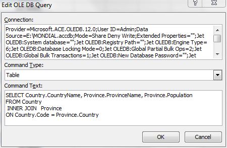
Here’s a very simple example using my trusty pie data. In this example I have two different tables on two sheets with slightly different pie orders. Here’s the output from data warehouse 1…

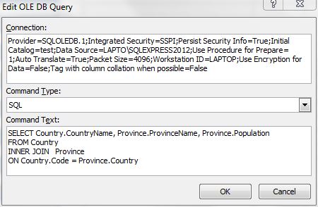
and here it is from data warehouse 88b…

I conveniently placed differences in the Quantity column near the top, so you may be able to just pick them out by eye. And you may even have caught the one date field discrepancy. However, after combining the two tables into one, adding a “Source” column and then pivoting, the differences become easy to pick out, especially with a little conditional formatting:

In the pivot above, “2”s in the Grand Total column represent all the records where the two queries returned the same results. The “1”s point to the discrepancies.

This is a flexible and powerful comparison method. Benefits include:

You can quickly add or subtract fields from the pivot to pinpoint the differences.
You can change the orders of the fields.
If you add subtotals you can then double-click on those with disrepancies to drill down to just those results.

For a while I created these combined source tables manually, just pasting the two sets of results together, adding a column “Source” column with “DW_1” and “DW_88b.” This worked fairly well, but after several times it cried out for automation.

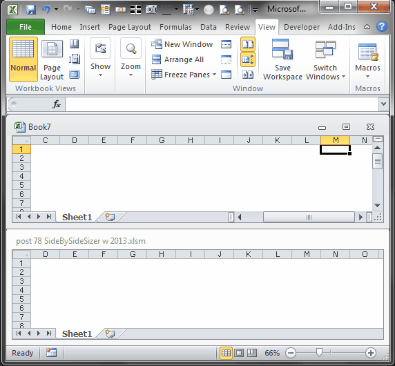
The VBA below keys off of selected sheets in a workbook. Just select the ones you want to pivot and then run the code. Here you can see that both sheets are selected, and I’ve added the “Pivot Multiple Sheets” macro to the tab’s right-click menu (with MenuRighter, of course).

The code first collects all the data necessary for the connection and then closes the source workbook. (I did this to avoid memory leaks or whatever it is that makes things go wonky if the workbook is open at the same time I’m creating a connection to it.) It uses that data to create the Source and SQL strings. The SQL is just a series of SELECTS, one for each selected worksheet, connected with UNION ALLs.

The newly created worbook contains a table with the connection to the source workbook and a pivot table pointed at that table. The table’s “Source” field becomes a column in the pivot table, containing the names of the two or more worksheets. The rest of the table columns become pivot table row fields. The connection in this workbook is live, so that if you make changes to the source they will appear in this workbook once you refresh the data and pivot:

Sub Pivot_Multiple_Sheets()

Dim wbToPivot As Excel.Workbook
Dim SheetsToPivot As Excel.Sheets
Dim SourceFullName As String
Dim SourceString As String
Dim wbWithPivot As Excel.Workbook
Dim wsWithQueryTable As Excel.Worksheet
Dim SheetsToPivotCount As Long
Dim SheetsToPivotNames() As String
Dim qt As Excel.QueryTable
Dim i As Long
Dim SqlSelects() As String
Dim sql As String
Dim pvt As Excel.PivotTable
Dim pvtField As Excel.PivotField

If ActiveWorkbook Is Nothing Then
MsgBox "No active workbook."
Exit Sub
End If
Set wbToPivot = ActiveWorkbook

If Not wbToPivot.Saved Then
MsgBox "Please save this workbook before running." & vbCrLf & _
"Workbook will be closed by this utility" & _
"after the process is completed."
Exit Sub
End If

'This code acts on the Selected Sheets
Set SheetsToPivot = wbToPivot.Windows(1).SelectedSheets
If SheetsToPivot.Count = 1 Then
MsgBox "Please select two or more worksheets (no charts)."
Exit Sub
End If

SheetsToPivotCount = SheetsToPivot.Count

For i = 1 To SheetsToPivotCount
If Not TypeName(SheetsToPivot(i)) = "Worksheet" Then
MsgBox "Please select two or more worksheets (no charts)."
Exit Sub
End If
Next i

SourceFullName = wbToPivot.FullName
ReDim SheetsToPivotNames(1 To SheetsToPivotCount)
For i = 1 To SheetsToPivotCount
SheetsToPivotNames(i) = SheetsToPivot(i).Name
Next i
'Change Selection to only one sheeet
SheetsToPivot(1).Select
'Close the source workbook before creating the new one and its connections
'Save it so not prompted
wbToPivot.Close True

Set wbWithPivot = Workbooks.Add
'Delete any extra worksheets
For i = wbWithPivot.Worksheets.Count To 2 Step -1
Application.DisplayAlerts = False
wbWithPivot.Worksheets(i).Delete
Application.DisplayAlerts = True
Next i
Set wsWithQueryTable = wbWithPivot.Worksheets(1)
wsWithQueryTable.Name = "Data Table"
'Don't know why this is needed, but otherwise .CommandText line below fails
wsWithQueryTable.Activate

'I got rid of a lot of fields in connection - still seems to work
SourceString = "ODBC;DSN=Excel Files;DBQ=" & SourceFullName
'Create an array of SELECT statements
ReDim SqlSelects(1 To SheetsToPivotCount)
For i = 1 To SheetsToPivotCount
SqlSelects(i) = "SELECT" & vbCrLf & _
"'" & SheetsToPivotNames(i) & "' as Source," & vbCrLf & _
"Sheet" & i & ".*" & vbCrLf & _
"FROM" & vbCrLf & _
"`" & SourceFullName & "`.[" & SheetsToPivotNames(i) & "$] AS Sheet" & i
Next i
'Connect the SELECTS with UNION ALL
For i = LBound(SqlSelects) To UBound(SqlSelects) - 1
sql = sql & SqlSelects(i) & vbCrLf & "UNION ALL" & vbCrLf
Next i
sql = sql & SqlSelects(i)

Set qt = wsWithQueryTable.ListObjects.Add(SourceType:=0, Source:=SourceString, Destination:=wsWithQueryTable.Range("$A$1")).QueryTable
With qt
.CommandText = sql
.ListObject.DisplayName = "tbl" & Format(Now(), "yyyymmddhhmmss") & Right(Format(Timer, "#0.00"), 2)
.RowNumbers = False
.FillAdjacentFormulas = False
.PreserveFormatting = True
.RefreshOnFileOpen = False
.BackgroundQuery = True
.RefreshStyle = xlInsertDeleteCells
.SavePassword = False
.SaveData = True
.RefreshPeriod = 0
.PreserveColumnInfo = True
'I like it to preserve the widths the first time it's run, and below turn it to false
.AdjustColumnWidth = True
.Refresh BackgroundQuery:=False
.AdjustColumnWidth = False
End With
wbWithPivot.Worksheets.Add
With ActiveSheet
.Name = "Pivot"
Set pvt = .Parent.PivotCaches.Create(SourceType:=xlDatabase, SourceData:=qt.ListObject.Name).CreatePivotTable(TableDestination:=.Range("A1"))
pvt.AddDataField Field:=pvt.PivotFields("Source"), Function:=xlCount
With pvt.PivotFields("Source")
.Orientation = xlColumnField
.Position = 1
End With
For Each pvtField In pvt.PivotFields
If pvtField.Name <> "Source" Then
pvtField.Orientation = xlRowField
pvtField.Position = pvt.RowFields.Count
End If
Next pvtField
End With
End Sub

To use this code put it in your Personal.xlsb or any workbook besides the one with the source data.

This code could use some more error-checking. For example, if the two sheets have a different number of columns. Even more important is the addition of whatever kind of general error handling you use so you exit gracefully from bad connection strings and other such inevitable problems.

Speaking of bad connection strings, you may notice that I’ve ditched the Default Directory, DriverId, BufferSize, MaxPageTimeOuts and whatnot from the connection. I did that to see if it worked. It did, so I never added them back. I see that they reappear in the connection properties for the table:

I ran this code in Excel 2010 and 2013. I don’t know how portable this code is to other Excel versions. I also don’t know if you’ll have performance issues if you have the source and pivot workbooks open at the same time.

If you’re interested in this topic be sure to take a look at Kirill Lapin’s method, posted on Contextures. His method keeps the source and the pivot table in one workbook, deleting the connection in between refreshes of the pivot table. I think Kirill’s method is nice for more traditional pivot table use where you want to merge different data sets with the same format, e.g., eastern and western sales regions.

I like my method because it requires no setup for the source workbook, keeps a refreshable connection and arranges the pivot table for comparison.

I’d love to hear anybody’s opinion on the stability of this method, i.e., when opening both the source and the connected data at the same time. Also, I’m curious if this code works in other versions besides 2010 and 2013. These are areas where my knowledge is pretty piecemeal, so any help would be appreciated.

MenuRighter Update!

Posted on April 11, 2015 by Doug Glancy

MenuRighter is my addin for modifying right-click menus, also known as context menus. It’s been around for three years and downloaded a few thousand times. It’s one of the cooler things I’ve ever made. I’ve just finished making some changes to it.

With MenuRighter you can turn this…

into this…

With four clicks I removed the Cut, Copy, Paste and Clear Contents buttons from the List Range Popup (Table) menu. With a few more I added my entire Personal Macro workbook (the cleverly named “myBar”) and its Tables sub-menu. Using MenuRighter’s new search functionality I quickly found and added two filter options along with the “Select Visible Cells” button.

Here’s what MenuRighter looks like. It’s divided into the Source menus and controls on the left and Target ones on the right. The Target menu is the one you’re adding controls to:

Removing and Adding Controls
And here’s a couple of quick videos showing how I did the deleting from, and adding to, in the Table context menu. This first one shows how to delete the controls – just select one and click Remove. For even faster removal you can double-click the control in the list:

Here I’m selecting the spot to insert the “Clear Selected Filter” and “Filter by Selected Cell’s Value” controls in the Target listbox. Then I filter in the Source combobox, click the Add button, and “hey Presto” they’re added. For even faster addition you can double-click the control to be added.

In both examples above, I clicked the “Apply Changes” button to actually modify the context menu. Up until then the “Reset to Current” button will revert the Target listbox to the context menu’s current setup. And at any time you can use the “Reset to Default” button to reset the menu back to Excel’s default.

Moving Controls

You can see in the clip above that controls are added above the selected control in the target menu. (If no control is selected the new control is added at the top. You can also use the Up, Down, Top and Bottom buttons to rearrange and controls in the target menu.

Settings

“But wait” I hear you say, “how did you know to choose to the “List Range Popup” menu to modify the context menu for a Table. The answer is MenuRighter’s handy “Show Labels on Menus” checkbox. It temporarily adds a control with the name and index to the bottom of each right-click menu.

There’s two other setting checkboxes. “Double-type dots” has to with MenuRighter convention for showing the Menu..Sub-menu..Control hierarchy. For instance, the Open control on the File is shown as Add Command..File..Open. If your search filter involves one of those “double-dots” I didn’t want you to have to type both, so, with that option checked, typing one dot gets you two.

The other Setting “Match Source Names” has to do with typing in the Source dropdown list at the top. That list contains all the toolbars that you can filter through in your search for controls. With the option checked, the combobox autofills the dropdown with the closest-matching item in the list. With it unchecked, it just filters based on whatever you type. It’s hard to describe, so just try it out.

The “Execute” Button
One other helpful new feature is the “Execute” button. When you’ve selected a control in the source list, and if that control is enabled, click Execute to run that control. For example, if you’ve selected Add Command..File..New and you click Execute, you’ll get a new workbook. (Pro Tip – choose the New command without three dots).

Search Tips

If you’ve used MenuRighter before, you’ll see that the main changes involve finding controls. The old version uses more of an Explorer type model of drilling down to controls. This new one lets you filter, with two big advantages: it’s faster and it’s more helpful if you have no idea where to start looking.

For example, the “filter by Selected Cell’s” value is a new control since 2003, so only shows in three context menus. Start typing “Filter by” into the Source combobox and you’ll see your choices instantly. On the other hand the Camera tool has been around (and hidden) forever. Type in “camera” and you’ve found it! “Freeze Panes” is another one that’s easy to find this way.

If you just want to scan through menus you can do it by scrolling through the seventy-or-so menus in the Source combobox. Or, you can choose menus in the Target combobox and click the “Show Current” button. Here’s an example of showing the Add Command controls. (Add Commands represents all the controls that were available in Excel 2003’s menu modification dialog):

Looking for A Few Testers

I’ll be posting this new version soon, but in the meantime it would be great to have a few folks try it out. If you’re interested please let me know in the comments section or through the contact form.

Tweaking View Side by Side

Posted on March 15, 2015 by Doug Glancy

I use View Side by Side a lot. That means I spend a bit of time fiddling with the two windows because I don’t always want each to take up half the space. I often make one smaller and then adjust the second to have it fill the rest of the screen. This weekend I set about tweaking View Side by Side to adjust one window when the other is resized.

Along the way I learned a few interesting things. The most important to this code was figuring out how tell if View Side by Side is activated. I also noticed some issues with View Side by Side in Excel 2013.

Below is a screenshot of what happens when you resize a window in View Side by Side. You can see that it needs to be followed up with some more fiddling to snug the lower window up against the upper one:

The code I came up with is in an application-level event. It uses a function to test whether View Side by Side is active. It’s designed to work in Excel 2010 (and 2007, although untested) as well as 2013. The 2013 tweaks were a little trickier, because Application.Height returned the same thing as Window.Height in 2013. This means the code needs to store the lower windows top location before resizing it.

You’ll also note that I used On Error Resume Next more freely than normally. After all we’re just resizing windows here, and it’s easier than testing for odd things like heights less than zero:

Public WithEvents app As Excel.Application

'application-level event in a class module
Private Sub app_WindowResize(ByVal Wb As Workbook, ByVal Wn As Window)
Dim UpperWindow As Excel.Window
Dim LowerWindow As Excel.Window
Dim OldLowerWindowTop As Double
Dim LowerWindowChange As Double

'See function below
If SideBySideOn Then
With Application
.EnableEvents = False
'assign the two windows,
'based on which is uppermost
If .Windows(1).Top <= .Windows(2).Top Then
Set UpperWindow = .Windows(1)
Set LowerWindow = .Windows(2)
Else
Set UpperWindow = .Windows(2)
Set LowerWindow = .Windows(1)
End If

'easy way to deal with heights less than zero, etc.
On Error Resume Next
'for Excel 2010 could just use Application.Height
'but in Excel 2013 each window is its own Application
If ActiveWindow.Caption = UpperWindow.Caption Then
OldLowerWindowTop = LowerWindow.Top
LowerWindow.Top = UpperWindow.Top + UpperWindow.Height
LowerWindowChange = LowerWindow.Top - OldLowerWindowTop
LowerWindow.Width = UpperWindow.Width
LowerWindow.Height = LowerWindow.Height - LowerWindowChange
Else
UpperWindow.Height = LowerWindow.Top
UpperWindow.Width = LowerWindow.Width
End If
On Error GoTo 0
.EnableEvents = True
End With
End If
End Sub

This code only responds to resizes involving the two horizontal borders in the middle, as well as the right-hand borders. So, if you drag the top border of the upper window nothing adjusts.

Application-Level Event

The sample workbook sets an application-level class in its Workbook_Open event. I’ve posted on this before and there’s lots of good info out there, like this Chip Pearson page.

How Do You Tell if View Side by Side is Active?

That’s an interesting question! Here’s what I tried:

First, I looked for some type of setting, like Application.ViewSideBySideEnabled. I can’t find one. Instead there’s two methods: CompareSideBySideWith and the rather drastic-sounding BreakSideBySide.
It would be nice if you could just get the state of the Ribbon’s View Side by Side button. That would tell you whether it’s active or not. But I don’t know of any way to do this.
You can, however, check the state of Excel 2003-style command buttons. So I tried looking at
Application.CommandBars(1).Controls("Window").Controls("Compare Side By Side With").State

to check whether it’s pressed. It turns out that control – ID 7698 – has no state. Instead it switches captions from “Compare Side by Side With” (followed by a workbook name if there’s only one choice) to “Close Side By Side.”
Based on #3 I considered getting the state by checking whether the first five letters are “Close” or “Compa.” But of course that wouldn’t work for folks with non-English Excel versions, and I generally shy away from using labels when I can use ID’s.
So, finally I decided to use the state of the “Reset Window Position” button. This button is only enabled when View Side by Side is active.

This leads to a one-line function that checks that button’s status using its ID of 7874. There is one final wrinkle, which is that this button doesn’t appear by default in the Excel 2003 “Window” toolbar. By default it lives only in the “Add Command” toolbar which was the one that appeared in 2003 when you modified a toolbar. No problem. We can find number 7874 wherever it lives by searching through all the commandbars using FindControl. Here’s the function:

Function SideBySideOn() As Boolean
'Reset Window Position
SideBySideOn = CommandBars.FindControl(ID:=7874).Enabled
End Function

Here’s how it looks with the code running:

Other Stuff Learned Along the Way

If you click the Reset Window Position button with the lower window selected, it moves to the top. I’d never noticed that.
There is no Window.Move event
View Side by Side in Excel 2013 is harder to use. This makes sense, since one of the biggest changes in Excel 2013 is the change to a Single-Document-Interface, making it easier to separate workbooks to multiple monitors. However it’s hard to grab the right edge of a workbook inside View Side by Side. And, as noted above, Application.Height and Window.Height now seem to be the same thing. This makes sense most of the time, but not when you are in View Side by Side mode and trying to compare the height of one of the workbooks/windows to the overall height.

Download!

Here you are my friend.

Get UNC Filenames

Posted on December 20, 2014 by Doug Glancy

If you work on a network with mapped servers or drives you may sometimes need a full UNC filename in it’s unmapped state. For example, computers in different departments may refer to the same location by different mappings. Say you work in the Pastry Procurement department and your computer refers to \\AcmeServer0023\Top_Secret_Pie_Recipes as T:\Top_Secret_Pie_Recipes, but your co-worker in Puddings and Pecan Puffs sees it as P:\Top_Secret_Pie_Recipes. If you send them a link using your mapping of “T:\” it won’t work for them. This post solves that problem by converting the mapped path – the one that starts with “T:\” – to its UNC equivalent – the one that starts with “\\AcmeServer0023.”

There are some fine methods out there for doing part of this conversion using VBA such as this comment by Emily at Daily Dose of Excel. That post also includes a method Dick discovered using the generally-reviled Web toolbar (I used to have a macro whose sole function was to hide that useless thing whenever it popped back up) but it only works for open workbooks.

This post incorporates existing Office functionality whereby links created with mapped drives actually show the UNC drive when you edit them. Here I’ve opened the Add Hyperlink dialog and selected a file. Note that the Address box at the bottom shows the mapped filename:

After closing the dialog and then opening the Edit Hyperlink dialog the Address box shows the UNC filename:

I like this method because it gives you the whole shebang and it works for all file types, not just Excel workbooks. Of course, it’s boring to generate more than a couple, so I wrote some VBA to automate the process. That way I can point to one or more files and paste their UNC monikers wherever I want.

This is a fairly trivial task and I’d rather not wipe out Excel’s Undo stack with the VBA. Since this hyperlink trick works just as well in Word, I thought I’d do it in a quickly opened, used, and then closed, instance of Word.

(You could modify this to open another Excel instance and use that, since you won’t lose the Undo stack across instances. You could also check if Word is already open and use that instance. I used Word because, since I don’t have addins in it, I think it opens faster. I don’t bother checking for an open instance because the whole thing only takes a couple of seconds as is.)

The code is pretty straightforward. It uses late binding for the Word objects, so that it doesn’t care what version of Word you’re using (and so that JP won’t give me grief if he’s still reading this blog). It also uses a Windows DataObject to hold the filenames and copy them to the clipboard.

Sub Browse_To_File_and_Copy_UNC_Names_to_Clipboard()
Dim fdFileDialog As FileDialog
Dim FileName As String
Dim FileNames As String
Dim doFileNames As DataObject
Dim SelectedItemsCount As Long
Dim wrdApp As Object
Dim wrdDoc As Object
Dim TempLink As Object
Dim i As Long

Set fdFileDialog = Application.FileDialog(msoFileDialogOpen)
With fdFileDialog
.ButtonName = "Select"
.FilterIndex = 1
.InitialView = msoFileDialogViewDetails
.Title = "Select Files"
.ButtonName = "Select"
.AllowMultiSelect = True
.Show
If .SelectedItems.Count = 0 Then
GoTo Exit_Point
End If
Set doFileNames = New DataObject
SelectedItemsCount = .SelectedItems.Count
Set wrdApp = CreateObject("Word.Application")
Set wrdDoc = wrdApp.Documents.Add
For i = 1 To SelectedItemsCount
Set TempLink = wrdDoc.Hyperlinks.Add(Anchor:=wrdApp.Selection.Range, Address:=.SelectedItems(i))
FileName = TempLink.Address
FileNames = FileNames & FileName & vbCrLf
Next i
FileNames = Left(FileNames, Len(FileNames) - 1)
doFileNames.SetText FileNames
doFileNames.PutInClipboard
End With

Exit_Point:
On Error Resume Next
wrdDoc.Close False
wrdApp.Quit
End Sub

When you run the code this dialog pops up. You can select one or more files:

After you’ve selected them, they’ll be in the Windows clipboard and you can paste them wherever you want, like into an email.

Importing SQL Files Into Data Connections

Posted on December 13, 2014 by Doug Glancy

By now you may know that I love data connections in Excel. Sometimes I use them for the front-ends in finished projects, but mostly I use them for testing SQL. With its formulas, tables and pivot tables, Excel makes a great test environment for validating SQL results. You can of course just paste query output straight from SQL Server Management Studio or other development environments, but the it doesn’t always format correctly. For instance Varchar ID fields that are all numbers lose leading zeros and dates lose their formats. In my experience those problems don’t happen with data connections

In this post, we’ll start with the basics of a reusable Table/SQL connection to which you can then add your SQL. Then I’ll share some code that lets you point at one or more .sql files and creates a connected table for each one. (An .sql file is just a text file with SQL in it and an .sql extension for handy identification.)

A Reusable Table/SQL Connection

At work I have a default data connection to the main database we query, all set up with the Connection, Command Type and some dummy Command Text. Whenever I want to run some SQL against that database in Excel, I just click on that connection in Data > Existing Connections. If I worked at home and used SQL Server and kept the corporate database on my laptop, the connection could look like this.

I created it by going to Data > Connections > Other Sources > From SQL Server. After following the wizard, I modified the connection by changing the Command Type to SQL and the Command Text to the meaningless, but super-speedy query “SELECT ‘TEMP’ FROM TEMP.”

So now I’ve got a template I can call from Data > Existing Connections and quickly modify the SQL, say to something like:

Inserting SQL Directly From .sql Files

Recently I thought I’d take this a bit further and pull the CommandText directly from an .sql file. So I wrote some code that has you pick one or more .sql files, and then creates a new Worksheet/Table/Query for each one in a new workbook. The main query is below. The heart of it looks a lot like what you got if you ran the macro recorder while creating a new connection:

Sub AddConnectedTables()
Dim wbActive As Excel.Workbook
Dim WorksheetsToDelete As Collection
Dim ws As Excel.Worksheet
Dim qt As Excel.QueryTable
Dim sqlFiles() As String
Dim ConnectionIndex As Long

sqlFiles = PickSqlFiles
If IsArrayEmpty(sqlFiles) Then
Exit Sub
End If

Workbooks.Add
Set wbActive = ActiveWorkbook
'Identify the empty sheet(s) the workbook has on creation, for later deletion
Set WorksheetsToDelete = New Collection
For Each ws In wbActive.Worksheets
WorksheetsToDelete.Add ws
Next ws

For ConnectionIndex = LBound(sqlFiles) To UBound(sqlFiles)
wbActive.Worksheets.Add after:=ActiveSheet
'*** Modify the location below to match your computer ***
Set qt = ActiveSheet.ListObjects.Add(SourceType:=0, _
Source:="ODBC;DSN=Excel Files;DBQ=E:\DOCS\YOURSUMBUDDY\BLOG\POST_72_SQL_IMPORTER\Post72_Data.xlsx;DriverId=1046;MaxBufferSize=2048;PageTimeout=5;", _
Destination:=Range("$A$1")).QueryTable
With qt
'Temporary command text makes the formatting for the real query work
.CommandText = ("SELECT 'TEMP' AS TEMP")
.ListObject.DisplayName = "tbl" & Format(Now(), "yyyyMMddhhmmss") & "_" & ConnectionIndex
.RowNumbers = False
.FillAdjacentFormulas = False
.PreserveFormatting = True
.RefreshOnFileOpen = False
.BackgroundQuery = True
.RefreshStyle = xlInsertDeleteCells
.SavePassword = False
.SaveData = True
.AdjustColumnWidth = True
.RefreshPeriod = 0
.PreserveColumnInfo = True
'Refresh first with just the template query
.Refresh BackgroundQuery:=False
.CommandText = ReadSqlFile(sqlFiles(ConnectionIndex))
'Refresh again with the new SQL. Doing this in two steps makes the formatting work.
.Refresh BackgroundQuery:=False
.AdjustColumnWidth = False
'Name the just-created connection and table
.ListObject.DisplayName = Replace("tbl" & Mid$(sqlFiles(ConnectionIndex), InStrRev(sqlFiles(ConnectionIndex), Application.PathSeparator) + 1, 99) & Format(Now(), "yyyyMMddhhmmss") & "_" & ConnectionIndex, ".sql", "")
wbActive.Connections(1).Name = .ListObject.DisplayName
End With
Next ConnectionIndex

'Delete the empty sheet(s) the worbook had on creation
Application.DisplayAlerts = False
For Each ws In WorksheetsToDelete
WorksheetsToDelete(1).Delete
Next ws
Application.DisplayAlerts = True
End Sub

Notice that the code refreshes the querytable twice. If I just go straight to the query from the .sql file, I end up with the same type of formatting problem described at the beginning of this post. For example, dates come through without formatting, like 41985. Starting with a dummy query of SELECT ‘TEMP’ AS TEMP, refreshing it, setting the .CommandText to the correct SQL and refreshing again results in correct formatting.

The code also sets .AdjustColumnWidth twice because I like to start with correct column widths and then not have them adjust after that.

You’ll also note that the connection in the code above isn’t to a SQL Server database anymore, but to an Excel workbook. That’s because I created a downloadable folder for you to try this out in, and the easiest data source to include is an Excel workbook. See the end of this post for the link and a few instructions.

(Also as a weird bonus in the code above is something I came up with to delete the one or more vestigial empty worksheets that get created in a situation like this where your creating a new workbook in code.)

Below are the three functions called from the module above. One uses a File Dialog to pick one or more .sql files.

Private Function PickSqlFiles() As String()
Dim fdFileDialog As FileDialog
Dim SelectedItemsCount As Long
Dim sqlFiles() As String
Dim i As Long

Set fdFileDialog = Application.FileDialog(msoFileDialogOpen)
With fdFileDialog
.ButtonName = "Select"
.Filters.Clear
.Filters.Add "SQL Files (*.sql)", "*.sql"
.FilterIndex = 1
.InitialView = msoFileDialogViewDetails
.Title = "Select SQL Files"
.ButtonName = "Select"
.AllowMultiSelect = True
.Show
If .SelectedItems.Count = 0 Then
GoTo Exit_Point
End If
SelectedItemsCount = .SelectedItems.Count
ReDim sqlFiles(1 To SelectedItemsCount)
For i = 1 To SelectedItemsCount
sqlFiles(i) = .SelectedItems(i)
Next i
End With
PickSqlFiles = sqlFiles

Exit_Point:
End Function

This one returns the SQL from the .sql file, so that it can then be stuffed into the QueryTable’s .CommandText property:

Private Function ReadSqlFile(SqlFileFullName As String)
Dim SqlFileLine As String
Dim Sql As String

Open SqlFileFullName For Input As #1
Do Until EOF(1)
Line Input #1, SqlFileLine
Sql = Sql & SqlFileLine & vbNewLine
Loop
'Sql = Input$ '(LOF(#1), #1)
Close #1
ReadSqlFile = Sql
End Function

And this is Chip Pearson’s code for checking if an array, specifically that returned by the PickSqlFiles function, is empty:

Public Function IsArrayEmpty(Arr As Variant) As Boolean
'Chip Pearson
Dim LB As Long
Dim UB As Long

Err.Clear
On Error Resume Next
If IsArray(Arr) = False Then
' we weren't passed an array, return True
IsArrayEmpty = True
End If
UB = UBound(Arr, 1)
If (Err.Number <> 0) Then
IsArrayEmpty = True
Else
Err.Clear
LB = LBound(Arr)
If LB > UB Then
IsArrayEmpty = True
Else
IsArrayEmpty = False
End If
End If
End Function

Download and Instructions

This download marks a new level of complexity, so it’s got instructions.

After you download you’ll need to unzip the folder to wherever you want. It contains five files, the xlsm with the code, the workbook data source and three .sql files with queries against that data source:

There’s further instructions in the xlam file. As noted there, you’ll need to change the path in the VBA to your unzipped folder (technically, you don’t because Excel will prompt you when it can’t find the folder in the VBA, but it will be cooler if you do). There’s a handy Cell formula in the Post72_Import_SQL.xlsm which will give you the correct file path.

Here’s the downloadable folder. Let me know what you think!

Undo Selections With SelecTracker!

Posted on November 6, 2014 by Doug Glancy

On one of the DDOE posts about International Keyboard Shortcut Day, a commenter known only as VvM asked for ways to undo selections in Excel. You know how it goes. You’ve selected various parts of a huge table to turn them bold or purple or something and you grab one more cell than you wanted. Wouldn’t it be great if you could just unselect it by clicking again, the way you can in just about any other #$;@#%! situation you can imagine. So, you keep clicking and it kind of looks like it worked because the active cell is a different color than the rest of the selection, but no. You’re doomed! You’ve got to start over from scratch. Aargh!

Anyways, the answer is there’s no way to undo selections in the Excel interface proper. You need VBA. And VBA is what you get in the handy form of my newest utility, SelecTracker.

Imagine you’re entered in a contest where you only have to click three cells with high dollar amounts to walk away with fistfuls of cash. Once you start you can’t start over, but you are allowed to use free utilities with goofy names that you downloaded from Excel websites (also with goofy names). In that case SelecTracker could really save your bacon:

That’s right. Just uncheck the offending selection(s) in the handy list and it’s like it never happened.

Other lovely SelecTracker features:

– Start it after your selections are made and you realize you need to unselect
– Doesn’t affect Excel’s Undo stack
– Gives you a better understanding of how Excel selections work

Weird Things I Learned About Selecting in Excel

Try this:

Hold down the Ctrl key and click A1 five times.

Now, in the Immediate window type:
? Selection.Areas.Count and hit Enter

Now enter:
? Selection.Address

So, all those times you tried to unselect by clicking again, you were really just selecting it even more. If only you’d had SelecTracker back then:

If you hold down the Ctrl key and click in cells A1 to A5 one at a time, you’ll get similar, slightly less weird, results. And if you do it and then start up SelecTracker (or vice-versa), you’ll see a different representation of the same results:

So, each selection (with a small “s”) in a Selection is a VBA Area. On the linked MSDN page the Areas definition reads:

The Areas collection contains one Range object for each discrete, contiguous range of cells within the selection.

But clearly that’s within the VBA world where Range("A1:A5") has one Area. But within a Selection (with a capital “S”) it has one Area for each selection you make while holding down the Ctrl key. “Contiguous” doesn’t really enter into it.

This makes the VBA pretty simple. To populate the form’s listbox, I just cycle through the Selection’s Areas and add each one:

With Me.lstSelections
.Clear
For Each SelArea In Selection.Areas
.AddItem SelArea.Address
.Selected(.ListCount - 1) = True
Next SelArea
End With

And to re-select the areas when a listbox item is checked or unchecked:

With Me.lstSelections
For i = 0 To .ListCount - 1
If .Selected(i) Then
NewSelection = NewSelection & .List(i) & ","
End If
Next i
NewSelection = Left(NewSelection, Len(NewSelection) - 1)
ws.Activate
ws.Range(NewSelection).Select
End With

I thought I’d do the above by Unioning the various Areas represented in the listbox. But once you Union them they’re not Areas any more. At least not if there contiguous. So instead I glued the text from the list items together.

(I don’t think other countries use other delimiters than commas, but can’t remember for sure and had no luck searching for it. Please tell me if you know otherwise.)

The rest of the code uses some concepts from UserForm Application-Level Events, Chip Pearson’s code for making forms resizable, and other neat stuff.

Download it and see for yourself.

Thanks VvM, whoever you are!

Four ListObject QueryTable Tests – Each Better Than the Last

Posted on May 15, 2014 by Doug Glancy

I started with this devil-may-care bit of code:

Sub Zero()
Dim ws As Excel.Worksheet
Dim lo As Excel.ListObject

For Each ws In ThisWorkbook.Worksheets
For Each lo In ws.ListObjects
On Error Resume Next
lo.QueryTable.Refresh
On Error GoTo 0
Next lo
Next ws
End Sub

Just wrap the QueryTable.Refresh in an On Error pair and don’t sweat it, that was my stance, at least for a day or two. If the ListObject had a QueryTable it would get refreshed. If it didn’t, it wouldn’t.

As the time got closer to hand it off to other people – people who might be bummed if their data didn’t refresh for reasons I hadn’t anticipated – I took a more prudent approach. I wrote some code to check if the ListObject actually had a QueryTable. This allows me to isolate the “ListOject with no QueryTable” error from all the others that might fly in under the radar.

I ended up with a simple function that’s now in my code library. But before we get to that, I’ll show you three lesser ListObject QueryTable tests, from bad to better:

#1 – Testing with Err.Number

In case you’re not familiar with On Error statements, I should clarify that On Error Resume Next let’s your code run willy-nilly through any and all errors. The madness only ends when an On Error Goto 0 statement is encountered. On Error Goto 0 also resets Err.Number to 0.

Sub One()
Dim ws As Excel.Worksheet
Dim lo As Excel.ListObject
Dim qt As Excel.QueryTable

For Each ws In ThisWorkbook.Worksheets
For Each lo In ws.ListObjects
On Error Resume Next
Set qt = lo.QueryTable
If Err.Number = 0 Then
qt.Refresh
End If
On Error GoTo 0
Next lo
Next ws
End Sub

I would never do this (not even in a really old Google Groups answer, I hope). It doesn’t fix the basic problem. The refresh is still happening with On Error set to Resume Next. It’s even worse if you have Else clauses. You could blunder through them as well before getting back to On Error Go To 0. The only way I can see it working is with another On Error Go To 0 right inside the IF clause before the refresh, and that’s just ugly.

#2 – Using an ErrorNum variable

Sub Two()
Dim ws As Excel.Worksheet
Dim lo As Excel.ListObject
Dim qt As Excel.QueryTable
Dim ErrorNum As Long

For Each ws In ThisWorkbook.Worksheets
For Each lo In ws.ListObjects
On Error Resume Next
Set qt = lo.QueryTable
ErrorNum = Err.Number
On Error GoTo 0
If ErrorNum = 0 Then
qt.Refresh
End If
Next lo
Next ws
End Sub

This approach fixes the problem in the previous routine by immediately setting an ErrorNum variable to Err.Number’s value. This tightens up the On Error Resume Next scope so it’s only active during the test. Pretty good, and for tests that don’t involve objects I’d probably stop there.

#3 – You’ve got an object variable, just use that!

Sub Three()
Dim ws As Excel.Worksheet
Dim lo As Excel.ListObject
Dim qt As Excel.QueryTable

For Each ws In ThisWorkbook.Worksheets
For Each lo In ws.ListObjects
Set qt = Nothing 'Don't forget this!
On Error Resume Next
Set qt = lo.QueryTable
On Error GoTo 0
If Not qt Is Nothing Then
qt.Refresh
End If
Next lo
Next ws
End Sub

Since we’re trying to set qt to something, let’s just test if it’s not nothing. This has the same advantage as the previous one: On Error statements bracket just the one line of your test, preventing stealth errors. The big gotcha is you’ve got to remember to set qt to Nothing before you try to set it to something. Otherwise, if the previous ListObject had a QueryTable, and this one doesn’t, the Resume Next will happily ignore the error and leave qt set to the previous one. That’s confusing, and potentially tragic.

#4 – The right way

Sub Four()
Dim ws As Excel.Worksheet
Dim lo As Excel.ListObject
Dim qt As Excel.QueryTable

For Each ws In ThisWorkbook.Worksheets
For Each lo In ws.ListObjects
Set qt = GetListObjectQueryTable(lo)
If Not qt Is Nothing Then
qt.Refresh
End If
Next lo
Next ws
End Sub

Function GetListObjectQueryTable(lo As Excel.ListObject) As Excel.QueryTable
On Error Resume Next
Set GetListObjectQueryTable = lo.QueryTable
End Function

Here I’ve moved the test into a function and put it in my utility module along with tests for workbook state, folder existence and other such mundanities. I know it works, I don’t have On Errors in the main module, and I only need Resume Next in the function, cause there’s not a heckuva lot of room for resuming.

Tangential miscellany

Here’s a pithy Jeff Weir rant on testing for ActiveCell.PivotTable versus ActiveCell.Listobject

This post deals with Excel-2007-and-on ListObject.QueryTables. In earlier versions QueryTables belonged to the worksheet they were on. In this Stack Overflow answer Dick (DDOE) Kusleika posts a function to find any QueryTable by name.

A thing I should know, but maybe you can tell me

What’s the difference between ListObject.Refresh and QueryTable.Refresh?

Listing UserForm Accelerator Keys

Posted on February 21, 2014 by Doug Glancy

Towards the end of the last post I showed a form I made to copy query properties from one table to another. That userform has 20 controls and, as always before I post something for your enjoyment, I tried to make is as user-friendly as possible.

So I set the default and cancel properties to the appropriate buttons and arrange the tab order of all the controls. When that’s done I assign accelerator keys to some of the controls. The accelerator property specifies a letter or other key, which when pressed along with the Alt key, activates that control.

In the example above, a helpful but peevish developer has specified the % key as the accelerator, perhaps for the first time in history.

I enjoy the fiddly work of setting tab orders and accelerators. I’d enjoy it more if the tab order dialog weren’t so hard to read.

It’s also hard to tell which controls have which accelerators and whether you’ve already used a certain letter.

So I wrote a bit of code that takes a userform as an argument and prints the relevant control properties to a newly-minted worksheet.

Sub ListUserFormAccelerators(frm As UserForm)
Dim ControlsCount As Long
Dim i As Long
Dim ctl As msforms.Control
Dim ControlName As String
Dim ControlTabIndex As Long
Dim ControlCaption As String
Dim ControlAccelator As String
Dim ControlProperties() As Variant
Dim ws As Excel.Worksheet
Const TableHeaders As String = "TabIndex,Name,Caption,Accerator,Count"

ControlsCount = frm.Controls.Count
ReDim ControlProperties(1 To ControlsCount, 1 To 4)
For i = 1 To ControlsCount
Set ctl = frm.Controls(i - 1)
ControlName = ctl.Name
ControlTabIndex = ctl.TabIndex
ControlCaption = ""
ControlAccelator = ""
'some controls don't have the next two properties
On Error Resume Next
ControlCaption = ctl.Caption
ControlAccelator = ctl.Accelerator
On Error GoTo 0
ControlProperties(i, 1) = ControlTabIndex
ControlProperties(i, 2) = ControlName
ControlProperties(i, 3) = ControlCaption
ControlProperties(i, 4) = ControlAccelator
Next i
Set ws = Workbooks.Add.Worksheets(1)
With ws
.Range("A1:E1") = Split(TableHeaders, ",")
.Range("A2").Resize(ControlsCount, 4) = ControlProperties
With .ListObjects.Add(xlSrcRange, .UsedRange, , xlYes)
.Name = "tblControlProperties"
.ListColumns("Count").DataBodyRange.FormulaR1C1 = "=COUNTIF([Accerator],[@Accerator])"
With .Sort
.SortFields.Add Key:=Range("tblControlProperties[TabIndex]")
.Header = xlYes
.Apply
End With
.Range.Columns.AutoFit
End With
'Want to close without prompt to save
.Parent.Saved = True
End With
End Sub

The code loops through a form’s controls and ultimately adds them all to an array which is dumped into a worksheet created in the code.

You’d call it like this:

Sub HereYouGo()
ListUserFormAccelerators frmCopyTableQuery
End Sub

And the result looks like this (click on it to open in its own, larger, window):

You may notice that some of the accelerators are doubled above. Each pair is for a label, followed by a textbox with no accelerator and then by a checkbox, which has the second occurrence of that acceelator. There’s two things going on here. The first is that if a control isn’t a Tab Stop, like a label, then the accelerator will take you to the next control, in this case the textbox. The second is that I wanted the user to be taken to the associated checkbox if they hit the accelerator again.

I can’t figure out how to call this code from another project. I messed around with Application.VBE.VBProjects, but can’t get it to work. Another nice thing would be the inverse of this code, a routine that would apply the tab order and accelerators from the worksheet to the userform.

Tables’ Edit Query Dialog

Posted on February 15, 2014 by Doug Glancy

One of my favorite Excel features is the Edit OLE DB Query dialog, where you can edit a table’s data connection and SQL. If you’re not familiar with table data connections, I’m talking about tables created by clicking something like “From Access” in the ribbon’s Data menu. Besides Access, you can connect to other databases, Excel files, the web, and who knows what else. Here’s a nice example of connecting to Access.

To get to the Edit OLE DB Query dialog, right-click in a table and choose “Table” then “Edit…”

Each time I do so I’m filled with child-like wonder at the ability to throw in a new connection string, switching, for example, from Access to SQL Server.

In addition you can change from the default Command Type of “Table” – which returns all the contents of a table, query or view – to “SQL,” which allows you to enter SQL directly into the Command Text box.

As far as I can tell this SQL can be as complex as what you would use directly in that type of database. For example, you can use With statements with a SQL Server connection.

That being said, and depending on my access privilegees, I try to limit the amount of SQL on the Excel side. If possible, I connect to an existing database view and then maybe filter it in the Command Text box. So with a SQL Server view called vwScoresAllYears, I might narrow the results with SQL like “SELECT * FROM vwScoresAllYears WHERE vwScoresAllYears.year IN (2012,2013).”

As cool as that is – and it is – it pales next to the ability to switch connections to a completely different type of database. One time we were porting a project from Access to SQL Server. The front end was a big old workbook with a data table pointing at an Access query. The table had lots of calculated columns and several pivot tables pointing at it. To do the switch, we could have created a new table pointing at the SQL Server view, rebuilt the calculated columns and pointed the pivot tables at it. Instead, I just switched the connection string so that it pointed at the SQL Server view. Since the output columns were exactly the same, the transition was barely noticeable. I just hit refresh and the SQL Server data poured into the table.

The following two pics show what I mean. The first connection is to an Access database…

The second connection is to a SQL Server database:

If you’re wondering, the connection shown in the first picture in this post is to another Excel workbook. In that case there are three worksheets serving as tables. The SQL looks a bit different, because when referring to Excel sheets or ranges, the names are surrounded in brackets, and followed by dollar signs in the case of sheets. If the idea of using SQL on Excel workbooks is new to you, this MSDN page is a good start.

I often find myself copying query settings from one table to another. For a while I’d open the Edit OLE DB Query dialog for a table, copy the connection data, open the dialog for the second one and paste the data. That got kind of boring, so guess what? That’s right, I wrote a tool to do what I want:

The way it works is you select a Source table – by clicking into a table and clicking the form button – and then do the same for the Target. You then select which parts of the query – Connection, Type, or Text – to copy over. You can also just edit the text in the Connection or Command Text boxes. Clicking the Copy button just copies the selected properties from the source side of the form to the target side – it doesn’t change the query properties themselves. You can make further edits in the target textboxes as needed. Clicking the Set Properties button copies applies the properties to the target table and attempts to refresh the table. If the refresh fails you get an error message. At that point you can tinker with the properties some more or click the Restore Last Good button, which will revert the table properties to the last working query.

This is different than the built-in dialog, which just reverts to the last working query. I find this ability to tweak a query until it works quite handy. Another advantage is that it opens up queries created by MS Query without the dialog telling you that you won’t be able to edit it.

To make it user-friendly for Dick and other shortcut-only types, the checkboxes can be reached by clicking the Alt Key combo for that property twice.

I uploaded an empty workbook that has a button to display this modeless form. If you download it be sure to save your work before trying this tool. I’ve used it for a few months now with no big issues, but better safe than sorry. Here’s the link.