Evaluate ActiveCell’s Table Row

Structured table references are pretty easy to generate in Excel. You know, the ones that look like:

Structured Reference

I recently realized you can use those structured references in a VBA Evaluate function to build strings based on the active row of a table. This makes for shorter code and avoids the use of Intersect, ListRow and ListColumn functions.

For example, let’s pretend you have a table of Oscar winners by year and you want to build a short sentence for each row of the table. Maybe you get a lot of emails from people asking what movie won the award in a given year. With a table like the one below you can simply choose the applicable row of column C and copy and paste it into your reply.

Per Row Output

This works okay, but it’s clunky. Instead, I’d rather generate the phrase in VBA based on the row of the ActiveCell. It was while writing this I had the happy thought to use VBA’s Evaluate function.

The Evaluate function basically returns the value of whatever you are evaluating as if it was entered in the active cell. At least that’s how I think of it for this instance. So, in the usage below, the structured reference’s @ symbol, e.g., [@Year] means “the value of the Year field in the active row of the table.”

It has two forms, one where you spell out Evaluate and one where you use square brackets, like I’ve done below.

Private Sub Worksheet_SelectionChange(ByVal Target As Range)
Dim BestPicString As String

'only proceed if the ActiveCell is in the table body
On Error Resume Next
If Intersect(ActiveCell, ActiveCell.ListObject.DataBodyRange) Is Nothing Then
   Exit Sub
End If
On Error GoTo 0

BestPicString = _
   ["Best Picture for " & tblBestPics[@Year] & CHAR(10) & "was " & tblBestPics[@Film]]
wsBestPics.Range("cellBestPic").Value = BestPicString
End Sub

Active Row Output to Cell

I did this because when I use the brackets I don’t have to double the quotes. I’m not absolutely sure of this, but here are the two versions of Evaluate that work for me:

BestPicString = Application.Evaluate _
   ("=""Best Picture for "" & tblBestPics[@Year] & CHAR(10) & ""was "" & tblBestPics[@Film]")

and

BestPicString = _
   ["Best Picture for " & tblBestPics[@Year] & CHAR(10) & "was " & tblBestPics[@Film]]

One more thing to note is that both versions error when I don’t include the table name – tblBestPics – although that’s not necessary in an actual Excel formula where you could just refer to [@Year].

Below is the code that I would write if I wasn’t using the Evaluate function. It’s not bad, but requires more variables and logic:

Sub Alternative()
Dim lo As Excel.ListObject
Dim ActiveTableRow As Long
Dim BestPic As String
Dim BestPicYear As String
Dim BestPicString As String

On Error Resume Next
If Intersect(ActiveCell, ActiveCell.ListObject.DataBodyRange) Is Nothing Then
   Exit Sub
End If
On Error GoTo 0

Set lo = ActiveCell.ListObject
'header row is DatabodyRange.Rows(0)
ActiveTableRow = ActiveCell.Row - lo.DataBodyRange.Rows(0).Row
BestPicYear = lo.ListColumns("Year").DataBodyRange.Rows(ActiveTableRow)
BestPic = lo.ListColumns("Film").DataBodyRange.Rows(ActiveTableRow)
BestPicString = "Best Picture for " & BestPicYear & vbCrLf & "was " & BestPic
wsBestPics.Range("cellBestPic").Value = BestPicString
End Sub

Workbook-level Listobject QueryTable Properties Manager

Here’s a utility I’ve used for years. It lets you manage True/False properties for structured tables with data connections – for example BackgroundQuery and PreserveColumnInfo. You can change properties for all tables in a workbook at once, or just one or a few tables.

ListObject QueryTable Properties Form

I only added some properties to the form. One of these, MaintainConnection, can’t be found in Excel’s front end, and the others appear in two different dialog boxes. So being able to change them for multiple tables in one dialog is really nice. For example, above I’d select all three tables using Ctrl-A and uncheck AdjustColumnWidth and MaintainConnection. You can see that currently both highlighted tables have AdjustColumnWidth turned off. Also, a gray checkmark, like the one for MaintainConnection, means that some selected tables have it turned on but others don’t.

Features

  • Select which tables to modify. Ctrl-A selects all tables in the workbook. The Choose Current Table button selects the table where the active cell is located.
  • The current settings for the selected tables are shown by the state of the checkboxes. The checkboxes are triple-state, so if the property is true for only some of of the selected tables, the checkmark will be gray, as with MaintainConnection in picture.
  • To change properties for selected tables, set them with the checkboxes, then click Apply.
  • Double-clicking a table activates the sheet it’s on.
  • To add another property to the VBA form, simply add a checkbox inside the grpProperties frame of the form. The checkbox caption must be the exact name of a Boolean property.

The VBA

I hadn’t looked at the VBA for this for a while, except to add MaintainConnection a year or so ago. The code was clunky in that it referred to each property individually in a couple of places, something like:

lo.QueryTable.MaintainConnection = me.chkMaintainConnection.Value
lo.QueryTable.BackgroundQuery = me.chkBackgroundQuery.Value

… and so on for each property/checkbox assignment.

I realized that CallByName would work great here. If you don’t know it, CallByName is kind of like an INDIRECT function for object properties and methods. So instead of the list above, I used something like this inside of a loop:

CallByName lo.QueryTable, ctl.Caption, VbLet, chk.Value
  • lo.QueryTable is the QueryTable object
  • ctl.Caption contains the property name, e.g., MaintainConnection
  • chk.Value is the value of the checkbox, i.e. True or False

To see the actual code and the working form go to the download link below.

A note about MaintainConnection

I’ve mentioned MaintainConnection a couple of times now. It’s the key to an issue that comes up once a year or so, and adding this property to the form helps me remember the solution.

The issue occurs when connecting a structured table to another workbook. If MaintainConnection is True and I refresh the table, it locks the source workbook and it can’t be edited. I tried changing the connection to read only and fiddling with other connection settings, but setting MaintainConnection to false solves the issue. And this form makes it easy to do for every table in the workbook.

Download

Here’s a sample workbook with the form and some tables to test it on. Let me know what you think!

Filter and Sort a Listbox With a Helper Table

I’ve been attempting to bend the Recent Files folder to my will for creating my own recent files form in Excel. My motivation is that Recent Files in Excel 2013 is one step further removed than in 2010. Now I’ve got a form that accesses all the Excel files in Windows Recent folder. I learned some interesting things putting it together, like how to extract a shortcut’s path in VBA. Even more interesting – instead of filtering and sorting the form’s main listbox using Like functions, arrays and collections, I just pull all the file data into a structured table and use it as the listbox’s source. When I want to sort or filter the listbox I just sort or filter the table and re-populate the listbox from the table. Much easier! No multi-dimensional array quicksorts or dictionaries required.

Recent Files form and table

In actual use, the sheet with the table is hidden (it’s in my utility addin), but above is a picture of the form and the table working together.

Background

The Windows Recent Files list is some kind of semi-virtual folder that contains a bunch of shortcuts to the files you’ve opened since, well, I’m not sure when. In my Windows 10 and Windows 7 computers the path

Environ("APPDATA")\Roaming\Microsoft\Windows\Recent

gets me there.

One interesting thing about the Recent folder is that it contains workbooks that you create with code, which isn’t necessarily true in Excel’s Recent list. It also contains addins.

The folder looks like this:

Recent Files folder

It’s chock-full of all kinds of shortcuts. At first I thought I’d just use a FileBrowserDialog with the filter set to .xls* but that doesn’t work because the file types are really all .lnk. You can enter “.xl” in the Search box in the upper right and it will filter to just Excel files, but I can’t find a way to get something into the Search box using VBA.

So next I just plunked all the filenames into a sheet and added hyperlinks to the files that still exist (just like Excel’s recent files list, the shortcuts can outlive the files):

Recent Files sheet

That kind of works, isn’t a great interface for something like this. The thing that really doesn’t work is that without VBA you can’t click multiple hyperlinks at once.

So instead I turned that table into the source for a listbox on a userform. It’s got columns showing whether the file has been deleted, its modified date and full path:

Recent Files form

Filtering and Sorting the Listbox using the Tables Sort and Filter Objects

There it is nicely filtered to files that haven’t been deleted and other stuff sorted from newest to oldest, etc. And in order to get those nicely sorted dates, I just turned on the macro recorder and fiddled with some table-sorting VBA that it generated. Here’s the routine for the click event for the date-sorting label:

Private Sub lblFIleSort_Click()
Dim SourceTable As Excel.ListObject

If Me.lblFIleSort.Caption = "Unsorted" Then
    Me.lblFIleSort.Caption = "A to Z"
ElseIf Me.lblFIleSort.Caption = "A to Z" Then
    Me.lblFIleSort.Caption = "Z to A"
ElseIf Me.lblFIleSort.Caption = "Z to A" Then
    Me.lblFIleSort.Caption = "A to Z"
End If
Me.lblDateSort = "Unsorted"

Set SourceTable = ThisWorkbook.Worksheets("RecentFiles").ListObjects("tblRecentFiles")
With SourceTable.Sort
    .SortFields.Clear
    .SortFields.Add Key:=SourceTable.ListColumns("File").Range, _
                    SortOn:=xlSortOnValues, _
                    Order:=IIf(Me.lblFIleSort.Caption = "A to Z", xlAscending, xlDescending), DataOption:=xlSortTextAsNumbers
    .Header = xlYes
    .Orientation = xlTopToBottom
    .Apply
End With
FillLstRecentFiles
End Sub

That’s some pretty simple sorting code for a three-column listbox! The code for filtering it by filename is even shorter:

Private Sub txtFileFilter_Change()
Dim SourceTable As Excel.ListObject

Set SourceTable = ThisWorkbook.Worksheets("RecentFiles").ListObjects("tblRecentFiles")
SourceTable.Range.AutoFilter Field:=3, Criteria1:="=*" & Me.txtFileFilter.Text & "*", Operator:=xlAnd
FillLstRecentFiles
End Sub

The last line of each sub above calls the FillLstRecentFiles subroutine, which plunks the visible rows in the helper table into the listbox:

Sub FillLstRecentFiles()
Dim SourceTable As Excel.ListObject
Dim VisibleList As Excel.Range
Dim SourceTableArea As Excel.Range
Dim SourceTableRow As Excel.Range
Dim Source() As String
Dim i As Long

Me.lstRecentItems.Clear
Set SourceTable = ThisWorkbook.Worksheets("RecentFiles").ListObjects("tblRecentFiles")
On Error Resume Next
Set VisibleList = SourceTable.DataBodyRange.SpecialCells(xlCellTypeVisible)
On Error GoTo 0
If VisibleList Is Nothing Then
    GoTo Exit_Point
End If
For Each SourceTableArea In VisibleList.Areas
    For Each SourceTableRow In SourceTableArea.Rows
        i = i + 1
        ReDim Preserve Source(1 To 3, 1 To i)
        Source(1, i) = SourceTableRow.Cells(1)
        Source(2, i) = SourceTableRow.Cells(2)
        Source(3, i) = SourceTableRow.Cells(3)
    Next SourceTableRow
Next SourceTableArea
'If there's just one row
If i = 1 Then
    Me.lstRecentItems.Clear
    Me.lstRecentItems.AddItem (Source(1, 1))
    Me.lstRecentItems.List(0, 1) = Source(2, 1)
    Me.lstRecentItems.List(0, 2) = Source(3, 1)
Else
    Me.lstRecentItems.List = WorksheetFunction.Transpose(Source)
End If

The main thing about the code above is that it cycles through the discontiguous Areas of the filtered table.

I’ve taken this code and added it to my main utility addin. Every time I open the utility it creates the sheet with the source table. When the form is closed the table gets deleted. It’s not terribly fast on a network when it first parses through all the files, so I don’t know how much I’ll actually use it. But I’m pretty sure I’ll be using listbox helper tables.

Have You Ever Used a Table Like This?

I’m curious whether you’ve ever used a table as a listbox helper like this. If so, how well did it work?

Download

Here’s a download so you can try it out . It also has some nifty code for getting a shortcut’s path and other treats as well.

download

Selection.ListObject and Selection.PivotTable

In recent posts about using VBA to work with filters I’ve used ActiveCell.ListObject to test whether I’m dealing with a filtered table or a filtered range. At one point it occurred that maybe I should be looking at the Selection’s ListObject instead. For various reasons that doesn’t work, but it made me wonder how Selection.ListObject gets evaluated. For example, what if it spans two tables? And, while we’re at it what about Selection.PivotTable?

To be clear, everything said about Selection in this post actually applies to the more general Range object. It’s just that Selection is the range I’m interested in.

Selection.PivotTable

Let’s start with Pivot Tables. Excel’s help actually says exactly how Range.PivotTable is handled:

Returns a PivotTable object that represents the PivotTable report containing the upper-left corner of the [Selection].

So,

Selection.PivotTable

returns an error with the selection below because its upper-left corner is outside the pivot:

pivot selection

But this selection will return the pivot table because the upper-left cell of the selection intersects the pivot table:

pivot selection 2

Selection.ListObject

The rules for ListObjects, or at least what I’m guessing are the rules, are different. There’s nothing I can find in Help, so here’s what I made up:

Returns the ListObject intersected by the Selection. If more than one ListObject intersects the Selection, the ListObject that was created earliest is returned.

None of the pivot table’s “upper-left corner” stuff. If the selection intersects the table, the table is returned. So below

Selection.Listobject

returns Table3.

listobject selection 1

When the Selection intersects multiple ListObjects, it looks to me like Selection.ListObject returns the one that was created earliest. With the selection below, that means that it returns Table1.

listobject selection 2

In Conclusion

Now I have even more reasons to never use Selection.ListObject or Selection.PivotTable! They’re both quirky, and I don’t think I could expect users to know that if they select more than one table, they’ll get the oldest one (or for that matter, that they’d get any one). And for a pivot table, it would be kind of fussy to insist the upper-left corner of the selection be in the pivot table.

I’m sticking with ActiveCell. I think that’s the way Range.PivotTable and Range.Selection should have been designed as well. In other words, like Range.PivotTable does, only using ActiveCell instead of the upper-left corner.

Filter Column By All Selected Values

Excel’s Filter by Selected Cell’s Value is a popular command, and for good reason. It’s a quick way to filter the data that you’re looking at. There are times when I’d like to take it one step further and filter by the values of multiple cells. So I wrote some code and added a “Filter By All Selected Values” item to my right-click menu. It works just like Filter by Selected Cells except you can select multiple cells.

Filter by All Selected Cells

Here’s the result:

filtered ccells

There’s one situation where this feature is especially handy: that’s when I need to see all instances in one column of items that match a single characteristic in another column. For instance, “I want to see all the pie orders from customers who have ordered Red Velvet Cheesecake.”

I could do this operation with a Countif formula like…

=COUNTIFS([Name],[@Name],[Pie],"Red velvet cheesecake")>0

and then filter to all the rows that return TRUE.

COUNTIFS filter

But this new routine allows me to do this without helper columns.

Here’s How

First, select “Red Velvet Cheesecake,” then right-click and choose the regular old Filter > Filter by Selected Cell’s Value. You’ll see all the rows with that value.

Filter Step 1

Next, select all the customers and run the “Filter by All Selected Values” code. This will filter the Customers column by only the three currently visible names. This is the part that I don’t see how to do easily without this code.

Filter Step 2

Finally, clear the filter from “Pies” that you set in the first step. The result will match that above with the COUNTIFS formula.

A Brief Commercial Announcement

If you’re wondering how I got those things in my context menu see the MenuRighter page.

The Code

The code I wrote works for tables and contiguous areas.

Sub Filter_By_All_Selected_Values()

Dim FilterValues() As String
Dim i As Long, j As Long
Dim ColNumberInFilterRange As Long
Dim FilterRange As Excel.Range
Dim InTable As Boolean
Dim CollUniqueValues As Collection
Const MAX_FILTER_CELLS As Long = 10000

'Make sure we don't select cells hidden by filter
With Selection.SpecialCells(xlCellTypeVisible)
    If Union(ActiveCell.EntireColumn, .EntireColumn).Address <> ActiveCell.EntireColumn.Address Then
        MsgBox "Only select from one column"
        Exit Sub
    End If
    If .Areas.Count = 1 And .Rows.Count = 1 Then
        MsgBox "Select more than one cell"
        Exit Sub
    End If
    If .Cells.Count > MAX_FILTER_CELLS Then
        MsgBox "Cannot select more than " & MAX_FILTER_CELLS & " cells."
        Exit Sub
    End If

    'Set the range to be filtered depending on whether it's a Table or not
    If Not ActiveCell.ListObject Is Nothing Then
        Set FilterRange = ActiveCell.ListObject.Range
        InTable = True
    Else
        Set FilterRange = ActiveCell.CurrentRegion
    End If
    If Union(Selection, FilterRange).Address <> FilterRange.Address Then
        MsgBox "Please make sure all cells are within the same table or contiguous area."
        Exit Sub
    End If

    'If not in a table and we're filtering a different area than currently filtered
    'then turn the existing AutoFilter off, so no error when the new area gets filtered.
    If Not InTable And ActiveSheet.AutoFilterMode Then
        If ActiveSheet.AutoFilter.Range.Address <> .CurrentRegion.Address Then
            ActiveSheet.AutoFilterMode = False
        End If
    End If

    'Try to add every selected value to a collection - only unique values will succeed
    Set CollUniqueValues = New Collection
    For i = 1 To .Areas.Count
        For j = 1 To .Areas(i).Cells.Count
            On Error Resume Next
            CollUniqueValues.Add .Areas(i).Cells(j).Text, .Areas(i).Cells(j).Text
            On Error GoTo 0
        Next j
    Next i
    'Transfer the collection to an array for the AutoFilter function
    ReDim Preserve FilterValues(1 To CollUniqueValues.Count)
    For i = LBound(FilterValues) To UBound(FilterValues)
        FilterValues(i) = CollUniqueValues(i)
    Next i
    'Determine the index of the column to be filtered within the FilterRange
    ColNumberInFilterRange = (.Column - FilterRange.Columns(1).Column) + 1
    FilterRange.AutoFilter Field:=ColNumberInFilterRange, Criteria1:=FilterValues, Operator:=xlFilterValues
End With
End Sub

How it Works

The first part of the code consists of a few checks to make sure the selection is more than one cell, is only in one column, and that you haven’t selected a huge number of cells. This last one is controlled by the MAX_FILTER_CELLS constant. I set it at 10,000, a number that ran with no noticeable delay.

After that the code checks whether the ActiveCell is in a table or not. In either case, it assigns the range to be filtered to the FilterRange variable. It then checks that all the currently selected cells reside within either the same table or contiguous area.

The code uses our old friend the “get unique items using a collection” trick. It then applies a filter to the FilterRange.

The trickiest part of the code was defining the conditions that require an Exit Sub, such as selecting in multiple columns. That’s mainly because something like “Selection.Columns.Count” only returns the count of columns in the first Area of a selection. The same thing applies to the Selection’s CurrentRegion. I got around these limitations by using Union and the fact that Selection.Address returns the address for all areas in the the selection.

Download

Here’s a workbook with the code and the pie orders table so you can easily try the filtering I did above.

Importing SQL Files Into Data Connections

By now you may know that I love data connections in Excel. Sometimes I use them for the front-ends in finished projects, but mostly I use them for testing SQL. With its formulas, tables and pivot tables, Excel makes a great test environment for validating SQL results. You can of course just paste query output straight from SQL Server Management Studio or other development environments, but the it doesn’t always format correctly. For instance Varchar ID fields that are all numbers lose leading zeros and dates lose their formats. In my experience those problems don’t happen with data connections

In this post, we’ll start with the basics of a reusable Table/SQL connection to which you can then add your SQL. Then I’ll share some code that lets you point at one or more .sql files and creates a connected table for each one. (An .sql file is just a text file with SQL in it and an .sql extension for handy identification.)

A Reusable Table/SQL Connection

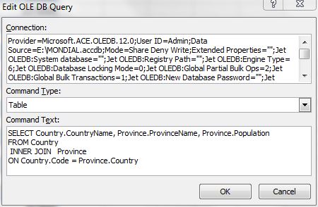
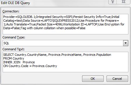
At work I have a default data connection to the main database we query, all set up with the Connection, Command Type and some dummy Command Text. Whenever I want to run some SQL against that database in Excel, I just click on that connection in Data > Existing Connections. If I worked at home and used SQL Server and kept the corporate database on my laptop, the connection could look like this.

SQL Server template connection

I created it by going to Data > Connections > Other Sources > From SQL Server. After following the wizard, I modified the connection by changing the Command Type to SQL and the Command Text to the meaningless, but super-speedy query “SELECT ‘TEMP’ FROM TEMP.”

So now I’ve got a template I can call from Data > Existing Connections and quickly modify the SQL, say to something like:

SQL Server template connection 2

Inserting SQL Directly From .sql Files

Recently I thought I’d take this a bit further and pull the CommandText directly from an .sql file. So I wrote some code that has you pick one or more .sql files, and then creates a new Worksheet/Table/Query for each one in a new workbook. The main query is below. The heart of it looks a lot like what you got if you ran the macro recorder while creating a new connection:

Sub AddConnectedTables()
Dim wbActive As Excel.Workbook
Dim WorksheetsToDelete As Collection
Dim ws As Excel.Worksheet
Dim qt As Excel.QueryTable
Dim sqlFiles() As String
Dim ConnectionIndex As Long

sqlFiles = PickSqlFiles
If IsArrayEmpty(sqlFiles) Then
    Exit Sub
End If

Workbooks.Add
Set wbActive = ActiveWorkbook
'Identify the empty sheet(s) the workbook has on creation, for later deletion
Set WorksheetsToDelete = New Collection
For Each ws In wbActive.Worksheets
    WorksheetsToDelete.Add ws
Next ws

For ConnectionIndex = LBound(sqlFiles) To UBound(sqlFiles)
    wbActive.Worksheets.Add after:=ActiveSheet
    '*** Modify the location below to match your computer ***
    Set qt = ActiveSheet.ListObjects.Add(SourceType:=0, _
        Source:="ODBC;DSN=Excel Files;DBQ=E:\DOCS\YOURSUMBUDDY\BLOG\POST_72_SQL_IMPORTER\Post72_Data.xlsx;DriverId=1046;MaxBufferSize=2048;PageTimeout=5;", _
        Destination:=Range("$A$1")).QueryTable
    With qt
        'Temporary command text makes the formatting for the real query work
        .CommandText = ("SELECT 'TEMP' AS TEMP")
        .ListObject.DisplayName = "tbl" & Format(Now(), "yyyyMMddhhmmss") & "_" & ConnectionIndex
        .RowNumbers = False
        .FillAdjacentFormulas = False
        .PreserveFormatting = True
        .RefreshOnFileOpen = False
        .BackgroundQuery = True
        .RefreshStyle = xlInsertDeleteCells
        .SavePassword = False
        .SaveData = True
        .AdjustColumnWidth = True
        .RefreshPeriod = 0
        .PreserveColumnInfo = True
        'Refresh first with just the template query
        .Refresh BackgroundQuery:=False
        .CommandText = ReadSqlFile(sqlFiles(ConnectionIndex))
        'Refresh again with the new SQL. Doing this in two steps makes the formatting work.
        .Refresh BackgroundQuery:=False
        .AdjustColumnWidth = False
        'Name the just-created connection and table
        .ListObject.DisplayName = Replace("tbl" & Mid$(sqlFiles(ConnectionIndex), InStrRev(sqlFiles(ConnectionIndex), Application.PathSeparator) + 1, 99) & Format(Now(), "yyyyMMddhhmmss") & "_" & ConnectionIndex, ".sql", "")
        wbActive.Connections(1).Name = .ListObject.DisplayName
    End With
Next ConnectionIndex

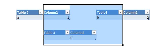
'Delete the empty sheet(s) the worbook had on creation
Application.DisplayAlerts = False
For Each ws In WorksheetsToDelete
    WorksheetsToDelete(1).Delete
Next ws
Application.DisplayAlerts = True
End Sub

Notice that the code refreshes the querytable twice. If I just go straight to the query from the .sql file, I end up with the same type of formatting problem described at the beginning of this post. For example, dates come through without formatting, like 41985. Starting with a dummy query of SELECT ‘TEMP’ AS TEMP, refreshing it, setting the .CommandText to the correct SQL and refreshing again results in correct formatting.

The code also sets .AdjustColumnWidth twice because I like to start with correct column widths and then not have them adjust after that.

You’ll also note that the connection in the code above isn’t to a SQL Server database anymore, but to an Excel workbook. That’s because I created a downloadable folder for you to try this out in, and the easiest data source to include is an Excel workbook. See the end of this post for the link and a few instructions.

(Also as a weird bonus in the code above is something I came up with to delete the one or more vestigial empty worksheets that get created in a situation like this where your creating a new workbook in code.)

Below are the three functions called from the module above. One uses a File Dialog to pick one or more .sql files.

Private Function PickSqlFiles() As String()
Dim fdFileDialog As FileDialog
Dim SelectedItemsCount As Long
Dim sqlFiles() As String
Dim i As Long

Set fdFileDialog = Application.FileDialog(msoFileDialogOpen)
With fdFileDialog
    .ButtonName = "Select"
    .Filters.Clear
    .Filters.Add "SQL Files (*.sql)", "*.sql"
    .FilterIndex = 1
    .InitialView = msoFileDialogViewDetails
    .Title = "Select SQL Files"
    .ButtonName = "Select"
    .AllowMultiSelect = True
    .Show
    If .SelectedItems.Count = 0 Then
        GoTo Exit_Point
    End If
    SelectedItemsCount = .SelectedItems.Count
    ReDim sqlFiles(1 To SelectedItemsCount)
    For i = 1 To SelectedItemsCount
        sqlFiles(i) = .SelectedItems(i)
    Next i
End With
PickSqlFiles = sqlFiles

Exit_Point:
End Function

This one returns the SQL from the .sql file, so that it can then be stuffed into the QueryTable’s .CommandText property:

Private Function ReadSqlFile(SqlFileFullName As String)
Dim SqlFileLine As String
Dim Sql As String

Open SqlFileFullName For Input As #1
Do Until EOF(1)
    Line Input #1, SqlFileLine
    Sql = Sql & SqlFileLine & vbNewLine
Loop
'Sql = Input$ '(LOF(#1), #1)
Close #1
ReadSqlFile = Sql
End Function

And this is Chip Pearson’s code for checking if an array, specifically that returned by the PickSqlFiles function, is empty:

Public Function IsArrayEmpty(Arr As Variant) As Boolean
'Chip Pearson
Dim LB As Long
Dim UB As Long

Err.Clear
On Error Resume Next
If IsArray(Arr) = False Then
    ' we weren't passed an array, return True
    IsArrayEmpty = True
End If
UB = UBound(Arr, 1)
If (Err.Number <> 0) Then
    IsArrayEmpty = True
Else
    Err.Clear
    LB = LBound(Arr)
    If LB > UB Then
        IsArrayEmpty = True
    Else
        IsArrayEmpty = False
    End If
End If
End Function

Download and Instructions

This download marks a new level of complexity, so it’s got instructions.

After you download you’ll need to unzip the folder to wherever you want. It contains five files, the xlsm with the code, the workbook data source and three .sql files with queries against that data source:

Unzipped folder

There’s further instructions in the xlam file. As noted there, you’ll need to change the path in the VBA to your unzipped folder (technically, you don’t because Excel will prompt you when it can’t find the folder in the VBA, but it will be cooler if you do). There’s a handy Cell formula in the Post72_Import_SQL.xlsm which will give you the correct file path.

Here’s the downloadable folder. Let me know what you think!

Copy an xlsm to an xlsx

This post features code I came up with to copy an xlsm to an xlsx. It has a few characteristics:

  • The code lives in the “master” workbook, i.e., the one that’s copied. It’s not in an addin.
  • The copy is an xlsx, stripped of any ribbon menus or VBA,
  • Tables in the master workbook are disconnected from any external data sources.
  • Any pivot tables pointing at tables in the master workbook are now pointing at their newly created copies in the copied workbook.
  • The copied workbook and master workbook are both still open after the code runs.

I looked at a few options when designing this system.

Creating a Workbook Copy
The most attractive choice for saving a copy of a workbook would seem to be the nicely named SaveCopyAs function, which keeps the master workbook open while saving a copy where you specify. Unfortunately, it won’t let you save in another format, so can’t be used to save an xlsm as an xlsx.

The second choice would be the SaveAs function, which does allow you to save in different formats. However, when you do the master workbook closes and the VBA stops running. Not impossible to work around, but I don’t like it.

Probably the best choice, at least in theory, is to run the process from an addin. Such an addin has application-level code to check whether you open any master workbooks. When you do, the ribbon menu is activated, with a button for copying the master. Since all the code is in the addin, the master workbook can be an xlsx and you can use SaveCopyAs. I’ve done a number of projects like this and they lend themselves to better coding practices, such as separating the presentation (pivot tables) from the code and the data. However, my project had just one user and the data sources are all external, so it’s simpler and quite maintainable to give them a workbook with both code and pivot tables. I hope.

So, what I’m actually using is ThisWorkbook.Sheets.Copy, which copies all the sheets. It has a few advantages. Since it’s only copying sheets the only code that gets copied would be in the ThisWorkbook or worksheet modules. I don’t have any so it’s not an issue. (The code would also get deleted when the workbook is saved as an xlsx, but I’m not sure if the user would be prompted about that when they close it). Likewise the ribbon tab, which in included in its own folder in the zip file that constitutes an xlsx or xlsm doesn’t get transferred.

There is one big issue with this method: since we’re copying individual sheets, albeit all of them all at once, any references to other worksheets still point at those worksheets in the master workbook. They don’t automatically transfer over to the new copies. In my case the only references to other sheets are pivot table sources – all other data is external. So I needed a way to point the pivot tables at their respective tables in the new workbook.

Fixing Pivot Table Data Sources

Again the the most appealing method, the pivot table’s ChangeConnection property, won’t work. It’s only for external connections, such as to a SQL Server database or web page. It doesn’t work for pivots connected to tables in the workbook.

My next idea was to modify the SourceData property for each PivotCache in the new workbook. According to Excel 2010 help, this is a read/write property, so it seems pretty straightforward to alter. After several attempts and some web searching I discovered it only works for pivot caches used by only one pivot table. If more than one pivot table points at a cache, PivotCache.SourceData isn’t your friend.

Happily, pivot tables also have a SourceData property. But, of course, there’s a catch here too. if you set two pivot tables’ SourceProperty to the exact same range, two pivot caches will be created. I want as few pivot caches as possible in a workbook, one for each distinct range.

So I came up with code that loops through each pivot table in the new workbook. First it calculates the string for the corrected data source, i.e., the external one with the workbook part stripped away. For example, if we remove the workbook part, e.g., “Master.xlsm”, from “Master.xlsm!tblPivotSource”, we get “tblPivotSource” which we can use to point at the correct table in the copied workbook.

As the code loops through the pivot tables it does one of two things:

  1. It sets the pivot table’s SourceData to the newly calculated NewSourceData variable. It only does this for the first pivot table with that source. Setting the SourceData creates a new pivot cache that uses the same SourceData.
  2. In each loop it first checks if there’s already a pivot cache with that source, which will be true if step 1 has already happened. If that’s the case, I set the pivot’s CacheIndex property to the index of that cache.

(Note that steps 1 and 2 happen in reverse order in the code, it’s just easier to describe them in this order.)

One very nice thing is that if a pivot cache no longer has any pivot tables pointing at it, that cache is automatically deleted.

The end result is that the copied workbook now has the same number of pivot caches as it started out with, each pointing at a table within the copied workbook. As mentioned earlier the listobjecs are also unhooked from their external connections.

Without further ado:

Sub CreateWorkbookCopy()
Dim wbWorkbookCopy As Excel.Workbook
Dim WorkbookCopyName As String
Dim ws As Excel.Worksheet
Dim lo As Excel.ListObject
Dim pvt As Excel.PivotTable
Dim pvtCache As Excel.PivotCache
Dim NewSourceData As String

Const SUBFOLDER_NAME As String = "Copied_Workbooks"

'Copies all worksheets, but not VBA or Ribbon
ThisWorkbook.Sheets.Copy

Set wbWorkbookCopy = ActiveWorkbook
With wbWorkbookCopy
    For Each ws In .Worksheets
        'Delete all listobject connections
        For Each lo In ws.ListObjects
            lo.Unlink
        Next lo
        'the pivot table caches are still pointing at ThisWorkbook, so
        'point them at wbWorkbookCopy
        For Each pvt In ws.PivotTables
            'note that the "!" is the delimiter between a workbook and table
            NewSourceData = Mid(pvt.SourceData, InStr(pvt.SourceData, "!") + 1)
            'if we just set the SourceData property we get a new cache for each sheet
            For Each pvtCache In wbWorkbookCopy.PivotCaches
                'if a previous loop has already re-pointed a pivot table,
                'then a new PivotCache with that SourceData has been created,
                'so just set the pivot table's cache to that
                If pvtCache.SourceData = NewSourceData Then
                    pvt.CacheIndex = pvtCache.Index
                Else
                    pvt.SourceData = NewSourceData
                End If
            Next pvtCache
        Next pvt
        'apparently PivotCaches are automatically deleted if no pivot tables are pointing at them
    Next ws

    If Not SubFolderExists(ThisWorkbook.Path & Application.PathSeparator & SUBFOLDER_NAME) Then
        MakeSubFolder ThisWorkbook.Path & Application.PathSeparator & SUBFOLDER_NAME
    End If
    WorkbookCopyName = Replace(ThisWorkbook.Name, ".xlsm", "") & "_copy_" & Format(Now(), "yyyy_mm_dd_hh_mm_ss") & ".xlsx"
    .SaveAs Filename:=ThisWorkbook.Path & Application.PathSeparator & SUBFOLDER_NAME & _
                      Application.PathSeparator & WorkbookCopyName, FileFormat:=51
End With
End Sub

For many useful functions involving pivot caches, please visit this wonderful Contextures page.

Irregular Banding for Repeated Values

A couple of years ago I came up with a formula to apply irregular banding for repeated values in a table or a pivot table. It uses conditional formatting and this SUMPRODUCT formula:

=MOD(SUMPRODUCT(($B$1:$B1<>$B$2:$B2)*1),2)=0

This array-type formula basically says: Count the number of times the value changes from one cell to the next up to the row where I am (assuming for a moment that I’m a cell). Divide that count by two, and check whether the remainder is 0. This True/False result can then be used to apply the conditional formatting.

The formatting looks like this, where the banding is based on changes in the Animal column:

irregular banding 1

If the above looks familiar, you may be thinking of this DDOE chestnut:

DDOE irregular bandingf

The difference, aside from my more subdued color scheme, is that Dick’s only starts a new band for the first hamster or what-have-you. It assumes (I assume) that each animal only has one group. Mine assumes bands of hamsters all over the place, and applies a new stripe with every change.

The bad news is my formula doesn’t do well in a long list if you try to delete large numbers of rows. For example, with 20,000 rows if I try to delete all but one, Excel goes into “Not Responding” mode longer than my patience will tolerate (roughly 35 seconds). I don’t know exactly why, but I bet if I re-read this Charles Williams post I would.

The other problem is, as John Walkenbach mentions in Dick’s post, the banding fails if you insert a line before the first row. I tried solving this by using INDEX (and OFFSET, I think) and learned you can’t use it in conditional formatting. Bummer.

The good news is neither of these problems affects its use in pivot tables.

So what to do if you’ve got a 20,000 rows of data you want to band irregularly? The answer, as Tushar Mehta pointed out, is a helper column:

irregular banding with helper column

Here’s the formula, starting in A2:

=IF(B2=OFFSET(B2,-1,0),OFFSET(A2,-1,0),SUM(OFFSET(A2,-1,0),1))

It uses the volatile OFFSET function. If you’re going to add or delete rows, OFFSET keeps you from getting #REF! errors or having gaps in the logic.

Then your conditional formatting formula is just: =MOD($A2,2)=0

One cool thing about the helper column banding formula above: It utilizes the fact that SUM ignores any text in the range you’re summing. If you get rid of the SUM and change it to =IF(B2=OFFSET(B2,-1,0),OFFSET(A2,-1,0),OFFSET(A2,-1,0)+1), you’ll get #VALUE! errors because of the text in A1.

Oh wow, look at the time. I’ve got to go restripe my parking lot. With these handy formulas it should go quickly though. See you soon!

art

Four ListObject QueryTable Tests – Each Better Than the Last

I started with this devil-may-care bit of code:

Sub Zero()
Dim ws As Excel.Worksheet
Dim lo As Excel.ListObject

For Each ws In ThisWorkbook.Worksheets
    For Each lo In ws.ListObjects
        On Error Resume Next
        lo.QueryTable.Refresh
        On Error GoTo 0
    Next lo
Next ws
End Sub

Just wrap the QueryTable.Refresh in an On Error pair and don’t sweat it, that was my stance, at least for a day or two. If the ListObject had a QueryTable it would get refreshed. If it didn’t, it wouldn’t.

As the time got closer to hand it off to other people – people who might be bummed if their data didn’t refresh for reasons I hadn’t anticipated – I took a more prudent approach. I wrote some code to check if the ListObject actually had a QueryTable. This allows me to isolate the “ListOject with no QueryTable” error from all the others that might fly in under the radar.

I ended up with a simple function that’s now in my code library. But before we get to that, I’ll show you three lesser ListObject QueryTable tests, from bad to better:

#1 – Testing with Err.Number

In case you’re not familiar with On Error statements, I should clarify that On Error Resume Next let’s your code run willy-nilly through any and all errors. The madness only ends when an On Error Goto 0 statement is encountered. On Error Goto 0 also resets Err.Number to 0.

Sub One()
Dim ws As Excel.Worksheet
Dim lo As Excel.ListObject
Dim qt As Excel.QueryTable

For Each ws In ThisWorkbook.Worksheets
    For Each lo In ws.ListObjects
        On Error Resume Next
        Set qt = lo.QueryTable
        If Err.Number = 0 Then
            qt.Refresh
        End If
        On Error GoTo 0
    Next lo
Next ws
End Sub

I would never do this (not even in a really old Google Groups answer, I hope). It doesn’t fix the basic problem. The refresh is still happening with On Error set to Resume Next. It’s even worse if you have Else clauses. You could blunder through them as well before getting back to On Error Go To 0. The only way I can see it working is with another On Error Go To 0 right inside the IF clause before the refresh, and that’s just ugly.

#2 – Using an ErrorNum variable

Sub Two()
Dim ws As Excel.Worksheet
Dim lo As Excel.ListObject
Dim qt As Excel.QueryTable
Dim ErrorNum As Long

For Each ws In ThisWorkbook.Worksheets
    For Each lo In ws.ListObjects
        On Error Resume Next
        Set qt = lo.QueryTable
        ErrorNum = Err.Number
        On Error GoTo 0
        If ErrorNum = 0 Then
            qt.Refresh
        End If
    Next lo
Next ws
End Sub

This approach fixes the problem in the previous routine by immediately setting an ErrorNum variable to Err.Number’s value. This tightens up the On Error Resume Next scope so it’s only active during the test. Pretty good, and for tests that don’t involve objects I’d probably stop there.

#3 – You’ve got an object variable, just use that!

Sub Three()
Dim ws As Excel.Worksheet
Dim lo As Excel.ListObject
Dim qt As Excel.QueryTable

For Each ws In ThisWorkbook.Worksheets
    For Each lo In ws.ListObjects
        Set qt = Nothing 'Don't forget this!
         On Error Resume Next
        Set qt = lo.QueryTable
        On Error GoTo 0
        If Not qt Is Nothing Then
            qt.Refresh
        End If
    Next lo
Next ws
End Sub

Since we’re trying to set qt to something, let’s just test if it’s not nothing. This has the same advantage as the previous one: On Error statements bracket just the one line of your test, preventing stealth errors. The big gotcha is you’ve got to remember to set qt to Nothing before you try to set it to something. Otherwise, if the previous ListObject had a QueryTable, and this one doesn’t, the Resume Next will happily ignore the error and leave qt set to the previous one. That’s confusing, and potentially tragic.

#4 – The right way

Sub Four()
Dim ws As Excel.Worksheet
Dim lo As Excel.ListObject
Dim qt As Excel.QueryTable

For Each ws In ThisWorkbook.Worksheets
    For Each lo In ws.ListObjects
        Set qt = GetListObjectQueryTable(lo)
        If Not qt Is Nothing Then
            qt.Refresh
        End If
    Next lo
Next ws
End Sub

Function GetListObjectQueryTable(lo As Excel.ListObject) As Excel.QueryTable
On Error Resume Next
Set GetListObjectQueryTable = lo.QueryTable
End Function

Here I’ve moved the test into a function and put it in my utility module along with tests for workbook state, folder existence and other such mundanities. I know it works, I don’t have On Errors in the main module, and I only need Resume Next in the function, cause there’s not a heckuva lot of room for resuming.

Tangential miscellany

Here’s a pithy Jeff Weir rant on testing for ActiveCell.PivotTable versus ActiveCell.Listobject

This post deals with Excel-2007-and-on ListObject.QueryTables. In earlier versions QueryTables belonged to the worksheet they were on. In this Stack Overflow answer Dick (DDOE) Kusleika posts a function to find any QueryTable by name.

A thing I should know, but maybe you can tell me

What’s the difference between ListObject.Refresh and QueryTable.Refresh?

Tables’ Edit Query Dialog

One of my favorite Excel features is the Edit OLE DB Query dialog, where you can edit a table’s data connection and SQL. If you’re not familiar with table data connections, I’m talking about tables created by clicking something like “From Access” in the ribbon’s Data menu. Besides Access, you can connect to other databases, Excel files, the web, and who knows what else. Here’s a nice example of connecting to Access.

To get to the Edit OLE DB Query dialog, right-click in a table and choose “Table” then “Edit…”

Each time I do so I’m filled with child-like wonder at the ability to throw in a new connection string, switching, for example, from Access to SQL Server.

Edit Query dialog 2

In addition you can change from the default Command Type of “Table” – which returns all the contents of a table, query or view – to “SQL,” which allows you to enter SQL directly into the Command Text box.

As far as I can tell this SQL can be as complex as what you would use directly in that type of database. For example, you can use With statements with a SQL Server connection.

That being said, and depending on my access privilegees, I try to limit the amount of SQL on the Excel side. If possible, I connect to an existing database view and then maybe filter it in the Command Text box. So with a SQL Server view called vwScoresAllYears, I might narrow the results with SQL like “SELECT * FROM vwScoresAllYears WHERE vwScoresAllYears.year IN (2012,2013).”

As cool as that is – and it is – it pales next to the ability to switch connections to a completely different type of database. One time we were porting a project from Access to SQL Server. The front end was a big old workbook with a data table pointing at an Access query. The table had lots of calculated columns and several pivot tables pointing at it. To do the switch, we could have created a new table pointing at the SQL Server view, rebuilt the calculated columns and pointed the pivot tables at it. Instead, I just switched the connection string so that it pointed at the SQL Server view. Since the output columns were exactly the same, the transition was barely noticeable. I just hit refresh and the SQL Server data poured into the table.

The following two pics show what I mean. The first connection is to an Access database…
Access connection

The second connection is to a SQL Server database:SQL Server connection

If you’re wondering, the connection shown in the first picture in this post is to another Excel workbook. In that case there are three worksheets serving as tables. The SQL looks a bit different, because when referring to Excel sheets or ranges, the names are surrounded in brackets, and followed by dollar signs in the case of sheets. If the idea of using SQL on Excel workbooks is new to you, this MSDN page is a good start.

I often find myself copying query settings from one table to another. For a while I’d open the Edit OLE DB Query dialog for a table, copy the connection data, open the dialog for the second one and paste the data. That got kind of boring, so guess what? That’s right, I wrote a tool to do what I want:

Copy Properties tool

The way it works is you select a Source table – by clicking into a table and clicking the form button – and then do the same for the Target. You then select which parts of the query – Connection, Type, or Text – to copy over. You can also just edit the text in the Connection or Command Text boxes. Clicking the Copy button just copies the selected properties from the source side of the form to the target side – it doesn’t change the query properties themselves. You can make further edits in the target textboxes as needed. Clicking the Set Properties button copies applies the properties to the target table and attempts to refresh the table. If the refresh fails you get an error message. At that point you can tinker with the properties some more or click the Restore Last Good button, which will revert the table properties to the last working query.

This is different than the built-in dialog, which just reverts to the last working query. I find this ability to tweak a query until it works quite handy. Another advantage is that it opens up queries created by MS Query without the dialog telling you that you won’t be able to edit it.

To make it user-friendly for Dick and other shortcut-only types, the checkboxes can be reached by clicking the Alt Key combo for that property twice.

I uploaded an empty workbook that has a button to display this modeless form. If you download it be sure to save your work before trying this tool. I’ve used it for a few months now with no big issues, but better safe than sorry. Here’s the link.