Formulas Archives - yoursumbuddy

Irregular Banding for Repeated Values

Posted on June 11, 2014 by Doug Glancy

A couple of years ago I came up with a formula to apply irregular banding for repeated values in a table or a pivot table. It uses conditional formatting and this SUMPRODUCT formula:

=MOD(SUMPRODUCT(($B$1:$B1<>$B$2:$B2)*1),2)=0

This array-type formula basically says: Count the number of times the value changes from one cell to the next up to the row where I am (assuming for a moment that I’m a cell). Divide that count by two, and check whether the remainder is 0. This True/False result can then be used to apply the conditional formatting.

The formatting looks like this, where the banding is based on changes in the Animal column:

If the above looks familiar, you may be thinking of this DDOE chestnut:

The difference, aside from my more subdued color scheme, is that Dick’s only starts a new band for the first hamster or what-have-you. It assumes (I assume) that each animal only has one group. Mine assumes bands of hamsters all over the place, and applies a new stripe with every change.

The bad news is my formula doesn’t do well in a long list if you try to delete large numbers of rows. For example, with 20,000 rows if I try to delete all but one, Excel goes into “Not Responding” mode longer than my patience will tolerate (roughly 35 seconds). I don’t know exactly why, but I bet if I re-read this Charles Williams post I would.

The other problem is, as John Walkenbach mentions in Dick’s post, the banding fails if you insert a line before the first row. I tried solving this by using INDEX (and OFFSET, I think) and learned you can’t use it in conditional formatting. Bummer.

The good news is neither of these problems affects its use in pivot tables.

So what to do if you’ve got a 20,000 rows of data you want to band irregularly? The answer, as Tushar Mehta pointed out, is a helper column:

Here’s the formula, starting in A2:

=IF(B2=OFFSET(B2,-1,0),OFFSET(A2,-1,0),SUM(OFFSET(A2,-1,0),1))

It uses the volatile OFFSET function. If you’re going to add or delete rows, OFFSET keeps you from getting #REF! errors or having gaps in the logic.

Then your conditional formatting formula is just: =MOD($A2,2)=0

One cool thing about the helper column banding formula above: It utilizes the fact that SUM ignores any text in the range you’re summing. If you get rid of the SUM and change it to =IF(B2=OFFSET(B2,-1,0),OFFSET(A2,-1,0),OFFSET(A2,-1,0)+1), you’ll get #VALUE! errors because of the text in A1.

Oh wow, look at the time. I’ve got to go restripe my parking lot. With these handy formulas it should go quickly though. See you soon!

Mod With no Zeroes

Posted on May 18, 2014 by Doug Glancy

I use both VBA’s and Excel’s Mod function occasionally, and many times I’ve wanted them to behave a little differently.

As described at its web page, the Mod function:

Returns the remainder after number is divided by divisor.

Mod is useful when you want to cycle through a group assigning repeating values to its members. It’s like when you go to a work training and have to count off by fours so you can break up into small groups and brainstorm or, preferably, when you go to the beach and have to come up with capture-the-flag teams. Here’s how it might look in Excel.

The thing is that the MOD function won’t give you quite that result, at least not without a little tweaking. Because it returns the remainder, the cycle always starts at one and ends at zero. So at your meeting it’s as if you asked people to count off like:

The solution is pretty simple (though it took me a while to figure out). Subtract one from the number you’re MODding, MOD it, and add one to the result. For example, in the worksheet above the formula in the Group column is:

=MOD(ROW()-2,4)+1

(We’re subtracting 2 because the names start in row 2)

Here’s a simple procedure in VBA to process that same list, using the same manipulation of MOD:

Sub GroupAttendees()
Dim ws As Excel.Worksheet
Dim i As Long
Dim Attendees As Variant
Dim GroupCount As Long

Set ws = ActiveSheet
Attendees = Application.Transpose(ws.ListObjects(1).ListColumns("Name").DataBodyRange)
GroupCount = 4
For i = LBound(Attendees) To UBound(Attendees)
Debug.Print Attendees(i); " "; ((i - 1) Mod GroupCount) + 1
Next i
End Sub

Here’s the results in the immediate window:

For a thorough discussion of Mod, including some gotchas, this page looks interesting.

Filter Pivot Tables Using Source Data Helper Columns

Posted on May 19, 2013 by Doug Glancy

When working with pivot tables you often need to filter out certain items. You can of course do this directly in the fields’ filter dropdowns, and often that’s good enough. But if you change the filters repeatedly this can be tedious and error-prone. For this reason, and to make my workbooks more flexible and maintainable, I often add helper columns to the source data. This post explains three types of source data helper columns that I use to filter pivot tables.

The live workbook below contains a simple data set of All-Star baseball games, where they were held, and which league won. It also contains three helper columns, each using a different method to determine the rows included in the pivot table. All three techniques refer to tables that spell out the criteria for inclusion.

(You can switch tabs, edit cells and refresh pivot tables. Reloading this page reverts it to its starting state. Note the buttons for downloading or opening in a full web page.)

You can click into the formulas in the helper columns and see that they are referring to tables – a different one for each column. Each formula uses a COUNTIF or COUNTIFS function to determine if the venue for that row meets certain criteria.

When you click on the “pivot and helper tables” tab you’ll see the pivot table on the left and the three helper tables on the right. The pivot table has a report filter for each of the three helper columns. Note that the report filters, table headers and helper columns are color-coded to show which ones go together.

Okay, let’s look at the three methods in order.

Table Containing Only Values to Include

Back on the data tab, the helper column “Venue In Table” looks at the first table, the one titled “Venues to Include”. The formula is a simple one:

=COUNTIF(tblVenuesToInclude[Venues to Include],[@Venue])>0

It returns TRUE if the ballpark for that row is found in the table. Its report filter is already set to TRUE in the pivot table, so you can test it by adding or deleting a stadium name in the table, right-clicking the pivot table and clicking “refresh”.

Table With All Values and an “Include” column

The second helper column/table pair are very similar, but instead of a table listing only the baseball fields you want included, you list all of them and add another column that contains TRUE if the ballpark should be included. I might use this method if I had a table with all the venues that I was already using for another purpose:

=COUNTIFS(tblVenuesIncludeCol[Venue],[@Venue],tblVenuesIncludeCol[Include],TRUE)>0

The COUNTIFS formula checks both the Venue and the Include columns. (You can use a SUMPRODUCT formula if you’re using Excel 2003 or earlier). You can test this formula by changing its report filter to TRUE and then changing the values in the Include column of the 2nd table.

Table Containing Words to Look For

The final helper column is “Venue Word in Table”. It looks into the “Word to Find” table and uses a COUNTIF array formula that searches the venue’s name for words from the table. Changing the report filter to TRUE will find the Kingdome, Polo Grounds and any park whose name contains “field”.

Here’s the formula, entered with Ctrl-Shift-Enter:

{=MAX(COUNTIF([@Venue],"*" & tblWordToFind[Word to Find] & "*"))>0}

This formula takes advantage of the ability to use wildcards in COUNTIF functions, by putting asterisks before and after the table column reference. Being an array formula, it tests the venue name against each word in the “Word to Find” table. The 1934 data row returns TRUE because “Polo Grounds” contains the word “polo”, which is in the table.

If we use the F9 key to successively evaluate parts of the function it looks like this:

=MAX(COUNTIF([@Venue],"*" & tblWordToFind[Word to Find] & "*"))>0

=MAX(COUNTIF([@Venue],"*" & {"king";"polo";"field"} & "*"))>0

=MAX(COUNTIF("Polo Grounds","*" & {"king";"polo";"field"} & "*"))>0

=MAX({0;1;0})>0

=1>0

TRUE

One final note: In actual practice, I always put the helper tables on a separate sheet, not next to the pivot table as done here. Expanding pivot tables, among other things, makes this layout impractical in real use.

No IFs in Conditional Formatting Formulas

Posted on March 14, 2013 by Doug Glancy

From time to time I’ll answer a question on Stack Overflow about a Conditional Formatting formula that includes an IF statement. Something like this:

=IF(A2=”Something”,TRUE,FALSE)

I’ll politely let them know you don’t need IFs in conditional formatting formulas, and that their formula can be reduced to something like:

=A2=”Something”

I’m going to go out on a limb and say there’s never a need for an IF in a conditional formatting formula.

Why “No IFs?”

What I usually say quickly in my answers is that the IF is implied by the fact that it’s a conditional formula. In other words, when you write the formula you’re telling the conditional formatting:

“If this condition is true, then apply the format, otherwise don’t apply it”. You only need the condition, the rest is a given.

Further, there will never be a reason for a nested IF. Nested IFs only apply when there are more than two possible outcomes. And again, in CF there can only be two: formatting applied or formatting not applied. You might very well, of course, use ORs and ANDs, as those allow you to narrow down the condition:

=AND(A2=”Something”,A3=”Else”)

But it’s still only one condition with two possible outcomes.

My Favorite F9 Trick

Posted on October 26, 2012 by Doug Glancy

I’ll let you know right now this trick is not real fancy, or even best practice, but it is my favorite F9 trick so I’m sharing it. It basically changes a variable in a formula to a constant.

I’ve mentioned before the handiness of F9 when creating formulas. Highlighting part of a formula and pressing F9 evaluates just that part of the formula, converting it to its result. So if you have “=1+2+3” and you hit F9 with “2+3” selected, the formula becomes “=1 + 5.”

Before I get to the trick, here’s a longer F9 example.

Imagine you are generating emails from a list of addresses and attachments. One of the columns contains the names of the files to attach. There can be one or more attachment names per cell, separated by commas. There’s also a master list of all the attachments to be sent.

To verify whether all the attachments were included exactly one time, you can use an array formula like this in column E:

{=SUM(ISNUMBER(
FIND("," & D3 & ",", "," & $B$2:$B$14 & ",")
)*1)=1}

If we highlight the 2nd row of that formula, in E3 and press F9 we get the following evaluation of the FIND section of the formula (with a few more #VALUE’s).

{#VALUE!;1;#VALUE!;#VALUE!;#VALUE!;#VAL …

FIND returns the position of the substring in the searched string, or #VALUE if the string isn’t found. The above tells us that the value in D3 is found once in B2:B14.

If you don’t already use F9, you should know that Ctrl-Z will undo the evaluation and return the formula to its formulaic state. You almost always want to do that, otherwise you’ll leave the hard-coded evaluation in the formula.

But not with my favorite F9 trick.

Even though it’s not a good practice in serious spreadsheets, sometimes I just want to hard-code a value into a formula. In these situations you can use F9 to insert the hard-coded value for you, and avoid typing errors. In this example, there’s a party with a randomized list of prizes for the guests.

So, column C has your formula to randomize the prize distribution. But, for reasons only known to you, you’ve decided the grand prize of a new car must go to Bahijah, and you want to hard-code that into your formula.

You could just type IF(B2=”Bahijah“, but to avoid spelling errors you instead select B13.

=IF(B2=B13,"New Car",
INDEX(Sheet1!$E$2:$E$10,
RANDBETWEEN(1,COUNTA(Sheet1!$E$2:$E$10))))

You then highlight B13 and press F9 and the beginning of the formula becomes:

=IF(B2="Bahijah","New Car",

Below, I used a table so that the formula would change in every cell in column C, and you can see the car become Bahijah’s in one fell swoop.

Curbside Recycling

Posted on September 26, 2012 by Doug Glancy

Here in my beloved hometown there are many things available for free out on the sidewalks. Often they are marked by a sign.

And often they’re not, like this whimsical offering of fake flowers and sparkly stuff.

I’ve been getting in on the act lately and have deposited various furnishings on the curb out front. I always put signs on them, and because I’m silly I always come up with different way to say “Free.”

My favorite so far is “Free to a good home … or yours.” A more convoluted sign said “The state I’ve achieved tastes of reality.”

If I was to do it in Excel I guess I’d go with “=PMT(0,1,0)“.

Preview Excel Custom Formats

Posted on September 16, 2012 by Doug Glancy

(Enter a format in column A and something in column B to preview the format.)

I was thinking of doing a simple post (hah!) on using Excel’s TEXT function to transform numbers to text, in order to match them to ID-type numbers from databases. One of my recurring work tasks is matching a host of possible school IDs from databases (text) to those in spreadsheets (numeric). I frequently use formulas like:

INDEX(tblFromCsv[School_Name],MATCH(TEXT(Numeric_ID,"0"),tblFromCsv[Text_Id],0))

Then recently a post here was featured on Chandoo’s site, along with some from other blogs – increasing my lifetime page views by about 30%. Searching his post for complimentary comments, I saw a couple along the lines of “Thanks for the great links, especially the one from Bacon Bits.”

Mike’s post is indeed a a beauty. It shows how to use custom number formats and create a percentage format like that shown in the first two rows of the interactive workbook above. It got me thinking about what formats you can specify in the TEXT function. It turns out anything you can enter as a custom format works for the TEXT’s Format argument, with very similar results. For example, this formula will format whatever’s in A1 with a format specified in B1:

=TEXT(A1,B1)

This got me thinking about creating a utility that shows the results of any custom format. Just like what you could get by using Excel’s custom format dialog or one line of VBA code, only a lot more work :). Although to be fair, Excel’s custom format dialog doesn’t show color:

The reason TEXT doesn’t show color is that Excel functions – native and user-defined – don’t change the format of a cell. TEXT may seem like it’s breaking that rule, but it just returns a string that mimics the specified formatting.

So, adding color without VBA became my ~~excuse~~ reason for creating this tool. To do so, I used conditional formatting and an additional 29 columns of formulas. You can check them out by scrolling right in the workbook above. (You can also download it by using the button at the bottom of the workbook.)

There are two general types of custom formats, so my first task was to determine which kind is being used. The first has four different conditions in the form:

Positive number formats; negative number formats; zero formats; text formats

You can use less than four conditions. If you use only one, negative numbers and zero will use the positive format. If you use two, then zeros get the positive format.

The second type of custom form is more free-form and allows you to enter two custom conditions, and corresponding formats, along with a third format that covers all conditions not met by the first two. The conditions are specified using comparison operators enclosed in brackets like “[=]” “[<>]” “[>]”, etc. The form is:

1st condition and formats; 2nd condition and formats; formats for unmet conditions

Rows 4 through 6 above have some examples. Keep in mind that these custom conditions are evaluated from left to right, and when one is met the evaluation stops, like a VBA If statement.

This Microsoft page has a good explanation of the conditional formats including both of these types.

Determining which of the two types is being is used pretty easy. If the format contains any comparison operators inside of brackets then “Has custom conditions” in column H is true. I used an array formula that searches the format for one of the operators listed in D15:D20:

{=IF($F2,SUM((ISERROR(SEARCH(main!$D$15:$D$20,main!A2))=FALSE)*1)>0,"")}

The rest of the 29 columns contain equally convoluted formulas that tease out the various conditions and whether they have associated colors. These are summarized in columns J:M and N:Q.

The conditional formatting uses COUNTIF. COUNTIF is the only function I know that understands comparison operators combined with numbers in a string. For example, if you have the numbers 1 to 10 in cells A1:A10 and “>5” in B1 you can do this:

So I ended up with a conditional format for each possible color, like this:

=INDEX(N2:Q2,MATCH(1,COUNTIF(B2,J2:M2),0))="[Red]"

It’s an array formula, but for some reason in conditional formatting you don’t have to enter them with Shft-Ctrl-Enter and you don’t get the curly brackets. If anybody knows how conditional formatting recognizes array formulas, I’d like to hear.

I know of two things that don’t work correctly in this tool:

Text is sometimes colored when it shouldn’t be. If a text color isn’t explicitly implied it should not be changed, unless the general format is used for the positive condition. With this tool it uses the positive condition format in all cases.
If you put a color or custom condition, things that are enclosed in brackets, inside of quotes, this will still recognize them as colors or conditions. So don’t do that, at least for testing.

I could fix the first, but I’m not sure about the second. If you see any other failings, feel free to leave a comment.

I mentioned that this all could be done with one line of code. Assuming you have a number in A1 and format in B1, this line of code will apply the format to the number. Note that you need to format B1 as text so you can enter formats like 0000 – without quotes – and not have Excel convert them to a single zero.

Range("A1").NumberFormat = Range("B1")

I learned a ton from doing this, and now have a much more detailed understanding of custom formats. Have you done any projects that were less-than-practical, but rewarding?

Index/Sumproduct or Index/Match for Multiple Criteria Lookups?

Posted on June 4, 2012 by Doug Glancy

You can use an INDEX/MATCH formula to look up an item in a list, as explained in this Contextures page. It’s trickier than a VLOOKUP formula, but it can look to the left and adjusts well when data columns are added or deleted. The generic layout of a single-criterion INDEX/MATCH is:

=INDEX(ColumnToIndex,MATCH(ItemToMatch, ColumnWithMatch, 0))

The MATCH section results in a row number that gets applied to the ColumnToIndex.

When looking up items with more than one criteria, I like to use an INDEX/SUMPRODUCT formula, replacing the MATCH part of the single criterion formula with SUMPRODUCT array multiplication, as descibed by Chandoo. Very generically that looks like:

=INDEX(ColumnToIndex,SUMPRODUCT(Multiply a bunch of columns and criteria))

This post started as an explanation of that approach. But in looking at the Contextures “INDEX/MATCH – Example 4” in the link above, I think it might be better. So this post is now a comparison of the two approaches.

Below is a live, downloadable worksheet with pairs of double-criteria lookup formulas – an INDEX/SUMPRODUCT and INDEX/MATCH in each case. Each row has two lookups: the first returns the number of home runs for that team and year, the second looks up a relative ranking.

I actually broke the formulas into two columns, which is what I’d do in a real project. Columns I and J contain INDEX formulas which refer to the lookup formulas in column H. The INDEX formulas first check if the lookup in column H actually returned a row. IF not “NA” is returned.

I break the lookup formula into two parts like this for a couple of reasons. The first is that if there’s no match the SUMPRODUCT in column H returns 0, which is important to see. The second is there’s often more than one formula referring to the calculated row, so it’s more efficient to only calculate it once and then use it in the different INDEX formulas. In this case the row is used for both the column I and column J INDEX formulas.

Here are the two lookup formulas, in cells H2 and H3, that are used to match the correct row. They are matching 2006 for the year and CHC for the team:

=SUMPRODUCT(($A$1:$A$33=$F2)*($B$1:$B$33=$G2)*(ROW($A$1:$A$33)-(ROW($A$1)-1)))
=MATCH(1,($A$1:$A$33=$F3)*($B$1:$B$33=$G3),0)

At their core they contain the same logic: ($A$1:$A$33=$F2)*($B$1:$B$33=$G2), which multiplies TRUEs and FALSES to return an array of Ones and Zeros. Here’s the SUMPRODUCT version with the above section evaluated by highlighting it and pressing F9. Note the 1 in the 19th position:

The SUMPRODUCT then multiplies that array times an adjusted row number, while the MATCH version finds the position of the number 1 in the array. Both result in row 19.

As mentioned above, the SUMPRODUCT formula returns 0 if no match is found. The INDEX formulas in columns I and J need to deal with that, otherwise they will return incorrect results. For example, if you have something like =INDEX({1,2,3,4,5},0), the result is 1. You might be surprised that it returns anything at all, but the nature of an INDEX formula is that if the row argument is set to 0 it evaluates the entire column. The actual row returned depends on the row of the formula. Confused? Me too.

The MATCH version, on the other hand, returns “#N/A” if no match is found, which is probably what you’d expect, and therefore good. And it’s shorter, also good. The only pitfall is that it’s an array formula and must be entered using Ctrl-Shft-Enter.

I’ve tried to make both sets of formulas more robust by including the headers in the ranges – $A1, $B1, etc. That way if a line in inserted below the header and before the first row of data, the formulas still work. I also want to ensure that the formulas still work if rows are inserted above the table’s header. This causes more complications in the SUMPRODUCT version, in the (ROW($A$1:$A$33)-(ROW($A$1)-1)) part. If you know the table will always start in Row 1 then it can be simplified to ROW($A$1:$A$33)-1. The MATCH version doesn’t have this issue.

Below the first pair of formulas are two more pairs, showing the results if no match is found, and if multiple matches are found. When there’s no match, the INDEX formula result in “NA” in both cases.

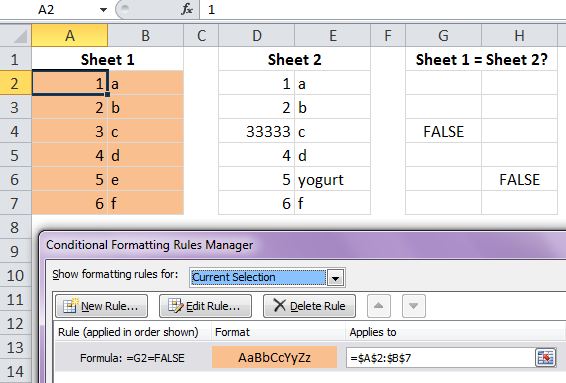
If there’s more than one match the SUMPRODUCT version adds together the matched rows. This results in 41 in row 12. Since 41 is outside the ColumnToIndex range, the result is #REF!. The MATCH version returns the first match. Obviously some kind of check for duplicates is good, such as the conditional formatting used here to highlight rows 20 and 21 of the data.

This being Excel, there are other ways to skin this cat. Here’s a post by JP Pinto, with his explanation of these two approaches, plus a LOOKUP version. (There’s a small error in the SUMPRODUCT version which is addressed in the comments.)

So which do I prefer now? Well, even though the MATCH version is simpler in most respects, I tend to avoid array formulas when possible, mainly because I too often forget that they are array formulas, do some editing, don’t hit Ctrl-Shft-Enter and have a moment, or several, of disorientation staring at the #N/A result. So I’ll probably stick with INDEX/SUMPRODUCT.

What do you think?

Oh You False Empty Cell

Posted on May 9, 2012 by Doug Glancy

I was comparing two worksheets by creating formulas off to the side of one sheet. These returned True if the corresponding cells in the two sheets matched, False if they didn’t. I converted the Trues and Falses to values, and replaced the Trues with nothing. Then I threw some conditional formatting on the data in one of the sheets. The formatting referred to the area with empty cells and Falses. The condition was for cells offset from Falses to be shaded.

I expected a smattering of color. What I got was a solid swath of light orange. Kind of like this, but on three separate sheets:

I assumed that I’d screwed up the conditional formatting formula, a not unreasonable premise. However, after a couple of minutes I was sure I hadn’t, and it was then I realized that empty cells equate to False. I’m sure everybody else already knows this, so I figured I’d better dig a little deeper in case it comes up at a party or something.

Next I checked if cells with =”” equate to False. They don’t. Neither do ones with 0, which I thought they might, since False multiplied by 1 equals 0. Here’s the visual summary, this time with a lambent blue for False.

In VBA the results are similar, except that 0 = vbEmpty. I have no idea what that means. I’m pretty sure Dick had a post on this, called “testing for empty cells,” but it seems to have gone down in the great DDOE server crash of 2011.

Solving the NPR Sunday Puzzle – #3

Posted on April 12, 2012 by Doug Glancy

Every time I hear Will Shortz say “name a country of the world” my heart beats a little faster, cause I know there’s probably an array-formula post in it. This week was no exception:

“Name an article of clothing that contains three consecutive letters of the alphabet consecutively in the word. For example, “canopy” contains the consecutive letters N-O-P. This article of clothing is often worn in a country whose name also contains three consecutive letters of the alphabet together. What is the clothing article, and what is the country?”

This spreadsheet is live. Double-clicking in a cell in the 2nd column shows the formula. You can then drag the lower-right fill handle to see the whole gnarly thing.

Countries are a lot more list-friendly, so I solved that part first. There are two types of solutions above: an array formula in the 2nd column, and a conditional formatting solution in the 3rd to 40-somethingth column. The 2nd solution is the way I’d do it for serious work, but the array formula is more fun:

=IFERROR(
MID(A4,MIN(IF(
CODE(MID(LOWER($A4),ROW(INDIRECT("1:"& LEN($A4)-2)),1))+1=
CODE(MID(LOWER($A4),ROW(INDIRECT("2:"& LEN($A4)-1)),1)),
IF(CODE(MID(LOWER($A4),ROW(INDIRECT("1:"& LEN($A4)-2)),1))+2=
CODE(MID(LOWER($A4),ROW(INDIRECT("3:"& LEN($A4))),1)),
ROW(INDIRECT("1:"& LEN($A4)-2))))),3),
"")

This formula says to compare every letter in the country name to the next two letters. If the numeric code for a letter is one less than the letter after it, and two less than the letter after that, return those three letters. The reason the 2nd column is mostly blank is because surprisingly few country names have three consecutive letters. (Or my formula sucks.)

Here’s how it works. Let’s assume the formula refers to Albania, the 3rd country in the list:

LEN returns the length of the country’s name.

INDIRECT(“1:”& LEN($A4)-2) evaluates to (1:5).

ROW(INDIRECT(“1:”& LEN($A4)-2)) evaluates to {1;2;3;4;5}. This tells the array formula which characters in “Albania” to evaluate against their respective two next characters. Using ROW this way is very handy in array formulas.

CODE(MID(LOWER($A4),ROW(INDIRECT(“1:”& LEN($A4)-2)),1)) resolves to {97;108;98;97;110}. In other words, the numeric values of the first five letters of Albania are 97, 108, etc. CODE is the function that returns the values. LOWER converts each letter to lower case, otherwise, for example, a lowercase “b” wouldn’t be seen as following an uppercase “A”. The MID piece tells the array formula to parse each of the first 5 letters in the word.

Okay, now we’re getting close. This bit:
CODE(MID(LOWER($A4),ROW(INDIRECT(“1:”& LEN($A4)-2)),1))+1=
CODE(MID(LOWER($A4),ROW(INDIRECT(“2:”& LEN($A4)-1)),1)) resolves to
{98;109;99;98;111}={108;98;97;110;105}, which in turn resolves to {FALSE;FALSE;FALSE;FALSE;FALSE}. In other words, one added to the code for the first five letters in “Albania” doesn’t ever equal the code for their respective next letters. So there’s not even two consecutive letters. What a country! The next two lines in the formula repeat the comparison, this time with the 2nd through 7th letters.

The 2nd line, which starts with MID, and the 2nd to last line say that if the whole mess is true, return the three letters that start at that position.

The IFERROR function at the beginning and the last line simply say that if the formula errors (doesn’t find three consecutive letters) put a blank in the cell. IFERROR is available in Excel 2007 and 2010. I like it very much as they keep formulas like this from being twice as ridiculously long.

Much of the evaluation above was done using the F9 key. Selecting part of a formula and then pressing F9 evaluates that piece of the formula, a very useful feature.

There are only two countries that meet the criteria, Afghanistan and Tuvalu. I figured it was probably the former and soon enough realized the article of clothing was “hijab.”

If you’ve made it this far, thanks! Oh yeah, the multiple cell and conditional formatting way works similarly to the array formula, only by breaking it up it’s a lot easier.

If anybody has a better array formula, please share.