Data Management Archives

Copy an xlsm to an xlsx

Posted on July 7, 2014 by Doug Glancy

This post features code I came up with to copy an xlsm to an xlsx. It has a few characteristics:

The code lives in the “master” workbook, i.e., the one that’s copied. It’s not in an addin.
The copy is an xlsx, stripped of any ribbon menus or VBA,
Tables in the master workbook are disconnected from any external data sources.
Any pivot tables pointing at tables in the master workbook are now pointing at their newly created copies in the copied workbook.
The copied workbook and master workbook are both still open after the code runs.

I looked at a few options when designing this system.

Creating a Workbook Copy
The most attractive choice for saving a copy of a workbook would seem to be the nicely named SaveCopyAs function, which keeps the master workbook open while saving a copy where you specify. Unfortunately, it won’t let you save in another format, so can’t be used to save an xlsm as an xlsx.

The second choice would be the SaveAs function, which does allow you to save in different formats. However, when you do the master workbook closes and the VBA stops running. Not impossible to work around, but I don’t like it.

Probably the best choice, at least in theory, is to run the process from an addin. Such an addin has application-level code to check whether you open any master workbooks. When you do, the ribbon menu is activated, with a button for copying the master. Since all the code is in the addin, the master workbook can be an xlsx and you can use SaveCopyAs. I’ve done a number of projects like this and they lend themselves to better coding practices, such as separating the presentation (pivot tables) from the code and the data. However, my project had just one user and the data sources are all external, so it’s simpler and quite maintainable to give them a workbook with both code and pivot tables. I hope.

So, what I’m actually using is ThisWorkbook.Sheets.Copy, which copies all the sheets. It has a few advantages. Since it’s only copying sheets the only code that gets copied would be in the ThisWorkbook or worksheet modules. I don’t have any so it’s not an issue. (The code would also get deleted when the workbook is saved as an xlsx, but I’m not sure if the user would be prompted about that when they close it). Likewise the ribbon tab, which in included in its own folder in the zip file that constitutes an xlsx or xlsm doesn’t get transferred.

There is one big issue with this method: since we’re copying individual sheets, albeit all of them all at once, any references to other worksheets still point at those worksheets in the master workbook. They don’t automatically transfer over to the new copies. In my case the only references to other sheets are pivot table sources – all other data is external. So I needed a way to point the pivot tables at their respective tables in the new workbook.

Fixing Pivot Table Data Sources

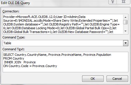
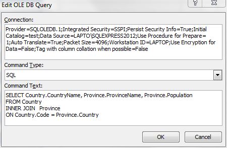
Again the the most appealing method, the pivot table’s ChangeConnection property, won’t work. It’s only for external connections, such as to a SQL Server database or web page. It doesn’t work for pivots connected to tables in the workbook.

My next idea was to modify the SourceData property for each PivotCache in the new workbook. According to Excel 2010 help, this is a read/write property, so it seems pretty straightforward to alter. After several attempts and some web searching I discovered it only works for pivot caches used by only one pivot table. If more than one pivot table points at a cache, PivotCache.SourceData isn’t your friend.

Happily, pivot tables also have a SourceData property. But, of course, there’s a catch here too. if you set two pivot tables’ SourceProperty to the exact same range, two pivot caches will be created. I want as few pivot caches as possible in a workbook, one for each distinct range.

So I came up with code that loops through each pivot table in the new workbook. First it calculates the string for the corrected data source, i.e., the external one with the workbook part stripped away. For example, if we remove the workbook part, e.g., “Master.xlsm”, from “Master.xlsm!tblPivotSource”, we get “tblPivotSource” which we can use to point at the correct table in the copied workbook.

As the code loops through the pivot tables it does one of two things:

It sets the pivot table’s SourceData to the newly calculated NewSourceData variable. It only does this for the first pivot table with that source. Setting the SourceData creates a new pivot cache that uses the same SourceData.
In each loop it first checks if there’s already a pivot cache with that source, which will be true if step 1 has already happened. If that’s the case, I set the pivot’s CacheIndex property to the index of that cache.

(Note that steps 1 and 2 happen in reverse order in the code, it’s just easier to describe them in this order.)

One very nice thing is that if a pivot cache no longer has any pivot tables pointing at it, that cache is automatically deleted.

The end result is that the copied workbook now has the same number of pivot caches as it started out with, each pointing at a table within the copied workbook. As mentioned earlier the listobjecs are also unhooked from their external connections.

Without further ado:

Sub CreateWorkbookCopy()
Dim wbWorkbookCopy As Excel.Workbook
Dim WorkbookCopyName As String
Dim ws As Excel.Worksheet
Dim lo As Excel.ListObject
Dim pvt As Excel.PivotTable
Dim pvtCache As Excel.PivotCache
Dim NewSourceData As String

Const SUBFOLDER_NAME As String = "Copied_Workbooks"

'Copies all worksheets, but not VBA or Ribbon
ThisWorkbook.Sheets.Copy

Set wbWorkbookCopy = ActiveWorkbook
With wbWorkbookCopy
For Each ws In .Worksheets
'Delete all listobject connections
For Each lo In ws.ListObjects
lo.Unlink
Next lo
'the pivot table caches are still pointing at ThisWorkbook, so
'point them at wbWorkbookCopy
For Each pvt In ws.PivotTables
'note that the "!" is the delimiter between a workbook and table
NewSourceData = Mid(pvt.SourceData, InStr(pvt.SourceData, "!") + 1)
'if we just set the SourceData property we get a new cache for each sheet
For Each pvtCache In wbWorkbookCopy.PivotCaches
'if a previous loop has already re-pointed a pivot table,
'then a new PivotCache with that SourceData has been created,
'so just set the pivot table's cache to that
If pvtCache.SourceData = NewSourceData Then
pvt.CacheIndex = pvtCache.Index
Else
pvt.SourceData = NewSourceData
End If
Next pvtCache
Next pvt
'apparently PivotCaches are automatically deleted if no pivot tables are pointing at them
Next ws

If Not SubFolderExists(ThisWorkbook.Path & Application.PathSeparator & SUBFOLDER_NAME) Then
MakeSubFolder ThisWorkbook.Path & Application.PathSeparator & SUBFOLDER_NAME
End If
WorkbookCopyName = Replace(ThisWorkbook.Name, ".xlsm", "") & "_copy_" & Format(Now(), "yyyy_mm_dd_hh_mm_ss") & ".xlsx"
.SaveAs Filename:=ThisWorkbook.Path & Application.PathSeparator & SUBFOLDER_NAME & _
Application.PathSeparator & WorkbookCopyName, FileFormat:=51
End With
End Sub

For many useful functions involving pivot caches, please visit this wonderful Contextures page.

Tables’ Edit Query Dialog

Posted on February 15, 2014 by Doug Glancy

One of my favorite Excel features is the Edit OLE DB Query dialog, where you can edit a table’s data connection and SQL. If you’re not familiar with table data connections, I’m talking about tables created by clicking something like “From Access” in the ribbon’s Data menu. Besides Access, you can connect to other databases, Excel files, the web, and who knows what else. Here’s a nice example of connecting to Access.

To get to the Edit OLE DB Query dialog, right-click in a table and choose “Table” then “Edit…”

Each time I do so I’m filled with child-like wonder at the ability to throw in a new connection string, switching, for example, from Access to SQL Server.

In addition you can change from the default Command Type of “Table” – which returns all the contents of a table, query or view – to “SQL,” which allows you to enter SQL directly into the Command Text box.

As far as I can tell this SQL can be as complex as what you would use directly in that type of database. For example, you can use With statements with a SQL Server connection.

That being said, and depending on my access privilegees, I try to limit the amount of SQL on the Excel side. If possible, I connect to an existing database view and then maybe filter it in the Command Text box. So with a SQL Server view called vwScoresAllYears, I might narrow the results with SQL like “SELECT * FROM vwScoresAllYears WHERE vwScoresAllYears.year IN (2012,2013).”

As cool as that is – and it is – it pales next to the ability to switch connections to a completely different type of database. One time we were porting a project from Access to SQL Server. The front end was a big old workbook with a data table pointing at an Access query. The table had lots of calculated columns and several pivot tables pointing at it. To do the switch, we could have created a new table pointing at the SQL Server view, rebuilt the calculated columns and pointed the pivot tables at it. Instead, I just switched the connection string so that it pointed at the SQL Server view. Since the output columns were exactly the same, the transition was barely noticeable. I just hit refresh and the SQL Server data poured into the table.

The following two pics show what I mean. The first connection is to an Access database…

The second connection is to a SQL Server database:

If you’re wondering, the connection shown in the first picture in this post is to another Excel workbook. In that case there are three worksheets serving as tables. The SQL looks a bit different, because when referring to Excel sheets or ranges, the names are surrounded in brackets, and followed by dollar signs in the case of sheets. If the idea of using SQL on Excel workbooks is new to you, this MSDN page is a good start.

I often find myself copying query settings from one table to another. For a while I’d open the Edit OLE DB Query dialog for a table, copy the connection data, open the dialog for the second one and paste the data. That got kind of boring, so guess what? That’s right, I wrote a tool to do what I want:

The way it works is you select a Source table – by clicking into a table and clicking the form button – and then do the same for the Target. You then select which parts of the query – Connection, Type, or Text – to copy over. You can also just edit the text in the Connection or Command Text boxes. Clicking the Copy button just copies the selected properties from the source side of the form to the target side – it doesn’t change the query properties themselves. You can make further edits in the target textboxes as needed. Clicking the Set Properties button copies applies the properties to the target table and attempts to refresh the table. If the refresh fails you get an error message. At that point you can tinker with the properties some more or click the Restore Last Good button, which will revert the table properties to the last working query.

This is different than the built-in dialog, which just reverts to the last working query. I find this ability to tweak a query until it works quite handy. Another advantage is that it opens up queries created by MS Query without the dialog telling you that you won’t be able to edit it.

To make it user-friendly for Dick and other shortcut-only types, the checkboxes can be reached by clicking the Alt Key combo for that property twice.

I uploaded an empty workbook that has a button to display this modeless form. If you download it be sure to save your work before trying this tool. I’ve used it for a few months now with no big issues, but better safe than sorry. Here’s the link.

ListBox Filter With Wildcards and Unique Values

Posted on September 2, 2013 by Doug Glancy

This post demonstrates a simple setup to filter a userform listbox as you type into a textbox. The filter uses VBA’s Like operator to pick up matches anywhere within the string. For example, typing “ursumb” matches to “yousumbuddy.” The Like operator allows wildcards, so “/*/201?” matches all dates from 2010 onwards. Like is also case-sensitive, so it can filter by case, or not, as specified. In addition the code uses the tried and true Collection method to allow filtering by unique items.

So, with this list of most popular US girls’ names for 2012 (modified in favor of “Emily”) you can filter and then add Unique and Case Sensitive filters. Note that clicking a name takes you to that row in the table:

Nice, isn’t it? Here’s the main routine, which gets called whenever the text in the filter textbox changes or one of the checkboxes is clicked:

Sub ResetFilter()
Dim rngTableCol As Excel.Range
Dim varTableCol As Variant
Dim RowCount As Long
Dim collUnique As Collection
Dim FilteredRows() As String
Dim i As Long
Dim ArrCount As Long
Dim FilterPattern As String
Dim UniqueValuesOnly As Boolean
Dim UniqueConstraint As Boolean
Dim CaseSensitive As Boolean

'the asterisks make it match anywhere within the string
FilterPattern = "*" & Me.txtFilter.Text & "*"
UniqueValuesOnly = Me.chkUnique.Value
CaseSensitive = Me.chkCaseSensitive

'used only if UniqueValuesOnly is true
Set collUnique = New Collection
Set rngTableCol = loActive.ListColumns(1).DataBodyRange
'note that Transpose won't work with > 65536 rows
varTableCol = Application.WorksheetFunction.Transpose(rngTableCol.Value)
RowCount = UBound(varTableCol)
ReDim FilteredRows(1 To 2, 1 To RowCount)
For i = 1 To RowCount
If UniqueValuesOnly Then
On Error Resume Next
'reset for this loop iteration
UniqueConstraint = False
'Add fails if key isn't UniqueValuesOnly
collUnique.Add Item:="test", Key:=CStr(varTableCol(i))
If Err.Number <> 0 Then
UniqueConstraint = True
End If
On Error GoTo 0
End If
'True if UniqueValuesOnly is false or if
'UniqueValuesOnly is True and this is the
'first occurrence of the item
If Not UniqueConstraint Then
'Like operator is case sensitive,
'so need to use LCase if not CaseSensitive
If (Not CaseSensitive And LCase(varTableCol(i)) Like LCase(FilterPattern)) _
Or (CaseSensitive And varTableCol(i) Like FilterPattern) Then
'add to array if ListBox item matches filter
ArrCount = ArrCount + 1
'there's a hidden ListBox column that stores the record num
FilteredRows(1, ArrCount) = i
FilteredRows(2, ArrCount) = varTableCol(i)
End If
End If
Next i
If ArrCount > 0 Then
'delete empty array items
'a ListBox cannot contain more than 65536 items
ReDim Preserve FilteredRows(1 To 2, 1 To Application.WorksheetFunction.Min(ArrCount, 65536))
Else
're-initialize the array
Erase FilteredRows
End If
If ArrCount > 1 Then
Me.lstDetail.List = Application.WorksheetFunction.Transpose(FilteredRows)
Else
Me.lstDetail.Clear
'have to add separately if just one match
'or we get two rows, not two columns, in ListBox
If ArrCount = 1 Then
Me.lstDetail.AddItem FilteredRows(1, 1)
Me.lstDetail.List(0, 1) = FilteredRows(2, 1)
End If
End If
End Sub

This routine takes advantage of the fact that Collection keys must be unique. If “Unique” is checked on the form, we test each value before adding it to the ListBox’s array.

The FilterPattern string has asterisks at the beginning and end. This is why the filter matches if it’s found anywhere within a table item.

In addition to the girl’s name, an array item also holds the record number for that name. This is used in another subroutine that activates the table row when the listbox selection changes:

Private Sub lstDetail_Change()
GoToRow
End Sub

Sub GoToRow()
If Me.lstDetail.ListCount > 0 Then
Application.Goto loActive.ListRows(Me.lstDetail.Value).Range.Cells(1), True
End If
End Sub

Here’s how it looks when filtering dates:

The speed is quite reasonable for tables with less than 10,000 items. Above that it gets slow, but is still usable all the way up to the limit of 65,536 listbox items. Yikes!

Here’s a workbook with all the code and the name and date tables to fool around with.

An Invitation

I’ve expanded this concept into a full-fledged Table Viewer. I’ve been using it in its alpha state and it’s quite handy for zipping around a big table. Along with the features here, it handles multiple columns, allows you to view only visible rows, and some other stuff. If anybody is interested in testing it out, leave a comment here or use the contact form.

Prompt to Add New Items to ComboBox or Data Validation

Posted on June 2, 2013 by Doug Glancy

Microsoft Access ComboBoxes have a handy NotinList event which allow you to check whether a value entered in a combobox is already in its list. If it’s not you can ask the user whether to add it. This post shows how to mimic that functionality in a combobox on a VBA userform. I also show how to do the same thing with a data validation list.

Creating a ComboBox NotInList Event

The key to doing this is checking the value of the ComboBox’s “MatchFound” property in its Exit event. If no match is found, we ask the user whether to add the item to the list of valid items (hats in this case). If the answer is “Yes” then a row with the hat is added to the table. If not, we clear the combobox and keep the focus on it. You can see this in action in the video above.

Here’s the code for the combobox’s Exit event:

Private Sub cboHats_Exit(ByVal Cancel As MSForms.ReturnBoolean)
Dim loValidationSource As Excel.ListObject
Dim loRow As Excel.ListRow

'the Table with the list of valid hats
Set loValidationSource = wsTables.ListObjects("tblValidationSource")
With Me.cboHats
'We're only interested if these aren't true
If .MatchFound Or .Value = "" Or .Value = STARTING_VALUE Then
Exit Sub
End If
'If the hat entered isn't in list, prompt to add it
If MsgBox(.Value & " is not in the list. Add it?", vbYesNo + vbDefaultButton2 + vbQuestion) = vbYes Then
Set loRow = loValidationSource.ListRows.Add
loRow.Range.Cells(1).Value = .Value
SortSourceTable
RefreshComboList
Else
'if "no", keep focus on the ComboBox and set it's value to "Choose a hat"
Cancel = True
Me.cboHats.Value = STARTING_VALUE
End If
End With
End Sub

One important thing is that the combobox’s “MatchRequired” property must be set to False (which is the default). Otherwise the Exit will be preempted by an “Invalid Property Value” message from Excel.

Creating a Data Validation NotInList Event

As with the combobox version, we use an event to prompt the user whether to add an item that’s not in the list. This time we use our own “MatchFound” function to check against the data validation’s source list. Similar to setting the “Match Required” combobox property to False, the data validation version requires that the “Show error alert after invalid data is entered” is unchecked in the data validation setup dialog. This is obviously not the default:

Since I’m working in Excel 2010, I’ve created a single-column table (listobject) to hold the valid items. I then simply pointed the data validation’s Source property at the column, excluding the header. Because the source is in a table, it’s dynamic – it adjusts when you add or remove items from the column. No dynamic ranges are required, just select the cells:

Here’s the code from the ThisWorkbook module, which contains the Workbook_SheetChange event and the MatchFound function:

Private Sub Workbook_SheetChange(ByVal Sh As Object, ByVal Target As Range)
Dim cell As Excel.Range
Dim loValidationSource As Excel.ListObject
Dim loHatCollection As Excel.ListObject
Dim loRow As Excel.ListRow

'wsTables is the sheet's CodeName
If Not Sh Is wsTables Then
Exit Sub
End If
Set loValidationSource = wsTables.ListObjects("tblValidationSource")
Set loHatCollection = wsTables.ListObjects("tblHatCollection")
'only continue if change is in column with data validation
If Intersect(Target, loHatCollection.ListColumns("Hat Type").DataBodyRange) Is Nothing Then
Exit Sub
End If
With Intersect(Target, loHatCollection.ListColumns("Hat Type").DataBodyRange)
For Each cell In .Cells
If MatchFound(cell.Value) = False And cell.Value <> "" Then
If MsgBox(cell.Value & " is not in the list. Add it?", vbYesNo + vbDefaultButton2 + vbQuestion) = vbYes Then
Set loRow = loValidationSource.ListRows.Add
loRow.Range.Cells(1).Value = cell.Value2
Else
cell.ClearContents
End If
End If
Next cell
End With
SortSourceTable
End Sub

Function MatchFound(ValueToCheck As Variant) As Boolean
Dim loValidationSource As Excel.ListObject
Dim ValidationList As Excel.Range

Set loValidationSource = wsTables.ListObjects("tblValidationSource")
Set ValidationList = loValidationSource.ListColumns("Hats Validation List").DataBodyRange
MatchFound = Application.WorksheetFunction.CountIf(ValidationList, ValueToCheck) > 0
End Function

And here’s what it looks like in action:

The Sort object – Excel 2007 Onwards

My code uses VBA’s Sort object, which appeared in Excel 2007. I like the way it works. You add Sort Fields, just as you do in the user interface, and then apply the sort when needed. If you are using Excel 2003 or earlier you’d need to re-write the two sorting procedures to work with your version.

Also, if you are using Excel 2003 or earlier, see this Contextures post for a non-table way of automatically adding items to a data validation list. You could easily add the code to prompt the user whether to do so.

Download

Here’s a workbook with all the code for both versions.

Filter Pivot Tables Using Source Data Helper Columns

Posted on May 19, 2013 by Doug Glancy

When working with pivot tables you often need to filter out certain items. You can of course do this directly in the fields’ filter dropdowns, and often that’s good enough. But if you change the filters repeatedly this can be tedious and error-prone. For this reason, and to make my workbooks more flexible and maintainable, I often add helper columns to the source data. This post explains three types of source data helper columns that I use to filter pivot tables.

The live workbook below contains a simple data set of All-Star baseball games, where they were held, and which league won. It also contains three helper columns, each using a different method to determine the rows included in the pivot table. All three techniques refer to tables that spell out the criteria for inclusion.

(You can switch tabs, edit cells and refresh pivot tables. Reloading this page reverts it to its starting state. Note the buttons for downloading or opening in a full web page.)

You can click into the formulas in the helper columns and see that they are referring to tables – a different one for each column. Each formula uses a COUNTIF or COUNTIFS function to determine if the venue for that row meets certain criteria.

When you click on the “pivot and helper tables” tab you’ll see the pivot table on the left and the three helper tables on the right. The pivot table has a report filter for each of the three helper columns. Note that the report filters, table headers and helper columns are color-coded to show which ones go together.

Okay, let’s look at the three methods in order.

Table Containing Only Values to Include

Back on the data tab, the helper column “Venue In Table” looks at the first table, the one titled “Venues to Include”. The formula is a simple one:

=COUNTIF(tblVenuesToInclude[Venues to Include],[@Venue])>0

It returns TRUE if the ballpark for that row is found in the table. Its report filter is already set to TRUE in the pivot table, so you can test it by adding or deleting a stadium name in the table, right-clicking the pivot table and clicking “refresh”.

Table With All Values and an “Include” column

The second helper column/table pair are very similar, but instead of a table listing only the baseball fields you want included, you list all of them and add another column that contains TRUE if the ballpark should be included. I might use this method if I had a table with all the venues that I was already using for another purpose:

=COUNTIFS(tblVenuesIncludeCol[Venue],[@Venue],tblVenuesIncludeCol[Include],TRUE)>0

The COUNTIFS formula checks both the Venue and the Include columns. (You can use a SUMPRODUCT formula if you’re using Excel 2003 or earlier). You can test this formula by changing its report filter to TRUE and then changing the values in the Include column of the 2nd table.

Table Containing Words to Look For

The final helper column is “Venue Word in Table”. It looks into the “Word to Find” table and uses a COUNTIF array formula that searches the venue’s name for words from the table. Changing the report filter to TRUE will find the Kingdome, Polo Grounds and any park whose name contains “field”.

Here’s the formula, entered with Ctrl-Shift-Enter:

{=MAX(COUNTIF([@Venue],"*" & tblWordToFind[Word to Find] & "*"))>0}

This formula takes advantage of the ability to use wildcards in COUNTIF functions, by putting asterisks before and after the table column reference. Being an array formula, it tests the venue name against each word in the “Word to Find” table. The 1934 data row returns TRUE because “Polo Grounds” contains the word “polo”, which is in the table.

If we use the F9 key to successively evaluate parts of the function it looks like this:

=MAX(COUNTIF([@Venue],"*" & tblWordToFind[Word to Find] & "*"))>0

=MAX(COUNTIF([@Venue],"*" & {"king";"polo";"field"} & "*"))>0

=MAX(COUNTIF("Polo Grounds","*" & {"king";"polo";"field"} & "*"))>0

=MAX({0;1;0})>0

=1>0

TRUE

One final note: In actual practice, I always put the helper tables on a separate sheet, not next to the pivot table as done here. Expanding pivot tables, among other things, makes this layout impractical in real use.