With formula-based conditional formatting, it’s pretty easy to base the formats on other cells in the workbook, simply by referring to those cells in the formula. However, it’s more complicated if you want color scales derived from values in another range. In this post I discuss two ways to base color scales on another range. The first uses the camera tool while the second is a VBA subroutine that mimics conditional formatting.
Below is an example of what I’m talking about. The color formatting isn’t based on the values in the pivot table. Instead, it reflects the values in the second table, each cell of which contains the difference from the previous year in the pivot table. The colors range from red at the low end to green at the high end:

So, here’s my two approaches to doing this:
Using the Camera Tool
This method uses Excel’s under-publicized camera tool, which creates a live picture linked to a group of cells. In this case the formatting is applied to a pivot table, but you can do it with any range. Here’s the steps:
- Create the range of formulas that you’ll base the conditional formatting on.
- Format the numbers in that range to be invisible, by using a custom format of “;;;”. All you want to see is the conditional formatting.
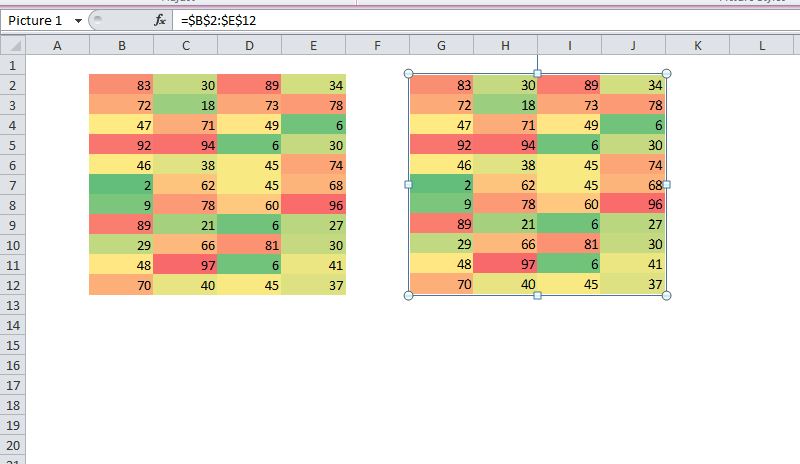
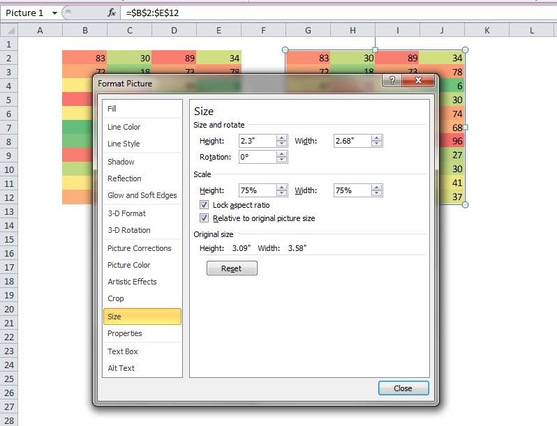
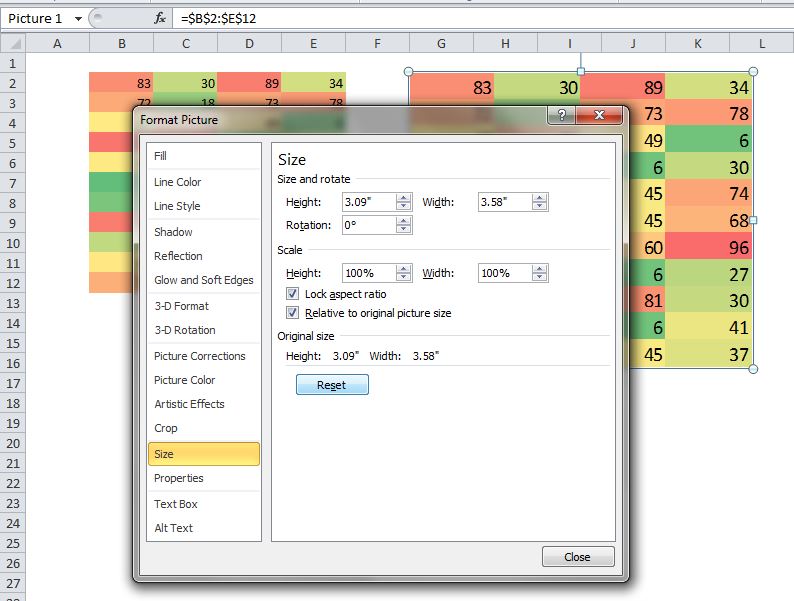
- Use the camera tool to take a picture of the entire pivot table and paste it over the range you just created, lining up the conditionally formatted cells. Set the picture to be completely transparent, using the “no fill” setting. This way you can see through the picture to the conditionally formatted cells underneath.
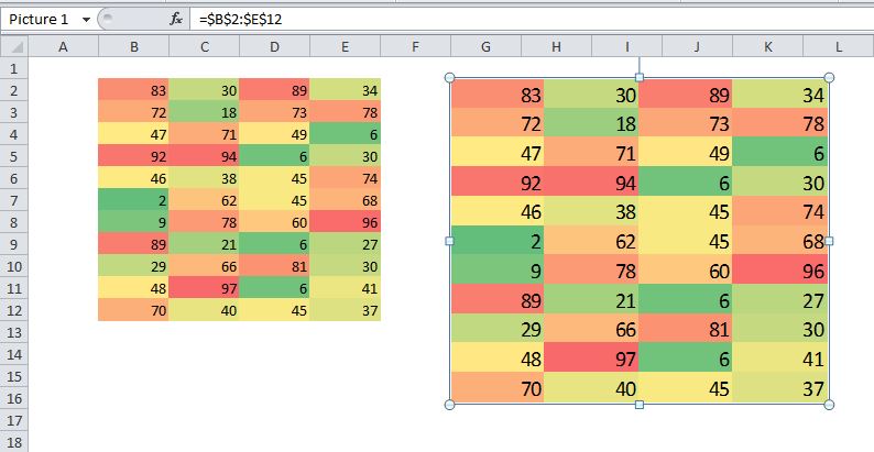
The result will be like the illustration below. The source pivot table is in rows 11 to 18, and you can see that the picture starting in row 2 is linked to it. The cells underneath the picture contain the formulas referring to the pivot table. The conditional formatting is based on these cells, whose text is invisible because of the custom format.

One thing to be aware of is that the picture doesn’t update until there’s a worksheet recalculation. You may have to force recalculation with F9 to have the picture update.
For one project I augmented this method by writing code that let me toggle back and forth between the values in the pivot table and the values the conditional formatting is based on.
Using VBA to Create “FauxMatting”
As the heading implies, this method attempts to replicate conditional formatting using VBA. The following subroutine takes two ranges – a source and a target range – as its arguments. It finds the highest and lowest values in the source range. It assigns each of those values a color in a scale from green to red, with white in the middle. This is done by dividing the range of values source values into 255 increments. The colors are then assigned to the target range:
Sub ConditionalFauxmatting(rngSource As Excel.Range, rngTarget As Excel.Range)
Const NUMBER_OF_INCREMENTS As Long = 255
Dim MinValue As Double
Dim MaxValue As Double
Dim ScaleIncrement As Double
Dim ScalePosition As Long
Dim var As Variant
Dim CellColor() As Long
Dim i As Long, j As Long
If Not (rngSource.Rows.Count = rngTarget.Rows.Count And rngSource.Columns.Count = rngTarget.Columns.Count) Then
MsgBox "Source and Target ranges must be" & vbCrLf & "same shape and size"
GoTo exit_point
End If
MinValue = Application.WorksheetFunction.Min(rngSource.Value)
MaxValue = Application.WorksheetFunction.Max(rngSource.Value)
'divide the range between Min and Max values into 255 increments
ScaleIncrement = (MaxValue - MinValue) / NUMBER_OF_INCREMENTS
'if all source cells have the same value or there's only one
If ScaleIncrement = 0 Or rngSource.Cells.Count = 1 Then
rngTarget.Cells.Interior.Color = RGB(255, 255, 255)
GoTo exit_point
End If
'assign all the values to variant array
var = rngSource.Value
ReDim CellColor(UBound(var, 1), UBound(var, 2))
For i = LBound(var, 1) To UBound(var, 1)
For j = LBound(var, 2) To UBound(var, 2)
'the scale position must be a value between 0 and 255
ScalePosition = (var(i, j) - MinValue) * (1 / ScaleIncrement)
'this formula goes from blue to red, hitting white - RGB(255,255,255) at the midpoint
CellColor(i, j) = RGB(Application.WorksheetFunction.Min(ScalePosition * 2, 255), _
IIf(ScalePosition < 127, 255, Abs(ScalePosition - 255) * 2), _
IIf(ScalePosition < 127, ScalePosition * 2, Abs(ScalePosition - 255) * 2))
Next j
Next i
'assign the colors stored in the array
'to the target range
With rngTarget
For i = 1 To .Rows.Count
For j = 1 To .Columns.Count
.Cells(i, j).Interior.Color = CellColor(i, j)
Next j
Next i
End With
exit_point:
End Sub
The result looks like this:

I’m not sure how practical this is, but it was fun to figure out! Obviously, you’d want to tie this to a worksheet or pivot table event to update the formatting when the values change.
Here’s a workbook demonstrating these two methods.